On Tuesday 24 November 1992 the European Centre for Medium-Range Weather Forecasts at Shinfield Park in Reading ran the first operational ensemble forecast in the history of medium-range weather prediction.1 The Cray Y-MP did not stop overnight; it merely produced thirty-three forecasts where it had previously produced one. The forecasts were identical in physics, identical in resolution, identical in everything except the initial conditions that fed them. Each had been seeded with a slightly different version of the atmospheric state for 00 UTC that morning, the differences being not random but carefully chosen along the directions in which a 48-hour forecast was most sensitive to small perturbations. The thirty-three forecasts ran out to T+240 hours – ten days – and were then dispatched to the European national weather services for whatever use they might be put to. Thirteen days later, on Monday 7 December 1992, the National Meteorological Center at Camp Springs in Maryland did approximately the same thing by a completely different method: fourteen forecasts a day at T62 resolution, each starting from a “bred” perturbation that had been growing through a chain of analysis cycles, integrated for twelve days on a Cray C90.2 Two operational centres, on opposite sides of the Atlantic, with two different recipes for the same conceptual move, launched the modern era of probabilistic weather forecasting in three weeks of late autumn 1992.
The shared intellectual debt was to one man at the Massachusetts Institute of Technology, Edward Norton Lorenz, then seventy-five years old and seven months past his birthday in May.3 Lorenz had argued in 1969 in Tellus that the atmosphere had a finite intrinsic predictability horizon of roughly two weeks, set by the upscale cascade of error from small unresolved scales to larger resolved ones, and that the conventional deterministic single forecast was for that reason an incomplete answer to the operational question.4 The right answer, Lorenz had argued, was a probability distribution over forecasts – a sample, however small, of the trajectories that the atmosphere might actually follow given the present analysis. Lorenz had not himself implemented an operational ensemble; he had spent the 1970s and 1980s thinking about the geometry of chaos in low-order models. The implementation came twenty-three years after the Tellus paper, in the three weeks of late 1992 covered by this post, from two teams that had been working largely independently toward the same destination.
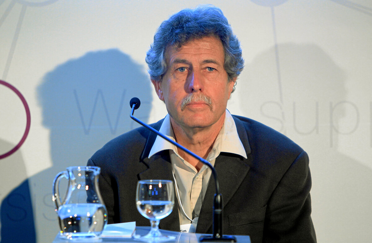
The European team was led by Professor Tim Palmer, then thirty-nine years old, head of the Predictability and Diagnostics Division at ECMWF, a division that had been created for him by the founding director Lennart Bengtsson in 1986.5 Working with him at Reading were two Italian theoretical physicists turned meteorologists – Franco Molteni, who had joined ECMWF in 1984 doing lagged-average forecasting experiments, and Roberto Buizza, who had computed the first primitive-equation singular vectors using the Integrated Forecasting System code – together with the Dutch researcher Robert Mureau, who led the experimental testing on the operational model, and the American Joe Tribbia on detail from the National Center for Atmospheric Research at Boulder, who had worked on the developing IFS tangent-linear and adjoint infrastructure.6 The five-person core had been at the ECMWF Ensemble Prediction System for six years by November 1992. Their method was the singular vector: an eigenvector of the tangent-linear forecast operator that maximised perturbation growth over a 48-hour optimisation window. Their computational requirement was substantial – the operational system needed a Lanczos iteration on the tangent and adjoint of the IFS at low resolution to extract the leading sixteen growing directions – and was the entire reason the system had taken six years to build.
The American team was led by Eugenia Kalnay, then fifty years old, the Director of the Environmental Modeling Center at NMC since 1987, the first woman ever to hold the position.7 Working with her at Camp Springs was the Hungarian post-Communist scientist Zoltan Toth, whom Kalnay had recruited around 1990, and the operational scientist M. Steven Tracton.8 Their method was the bred vector: a perturbation grown through the operational analysis-forecast cycle, periodically rescaled to keep its amplitude in the linear regime, asymptoting after many cycles to a structure resembling the dominant Lyapunov vector of the operational model. Their computational requirement was modest – two integrations of the nonlinear MRF model per bred direction, no adjoint code required – and was the entire reason the system had been deployed only thirteen days after ECMWF’s despite Kalnay having a noticeably smaller staff.
The two methods were not the same. They reflected different operational realities and different intellectual instincts about what mattered in the predictability problem. ECMWF, with the larger team and the larger machine, had spent six years building the linear-algebraic infrastructure needed to compute the eigenvectors of $\mathbf{A}^T \mathbf{A}$ for the operational forecast propagator $\mathbf{A}$, in the conviction that the right initial perturbations were the ones that grew fastest in a specified time. NCEP, with the smaller team and the smaller machine, had spent a much shorter time building a cyclic perturbation generator that needed only the nonlinear model and a rescaling step, in the conviction that the right initial perturbations were the ones the analysis cycle itself amplified. The two methods would dominate operational ensemble forecasting through the 1990s and most of the 2000s, with the European singular-vector lineage gradually gaining the edge on probabilistic skill scores and the American breeding lineage gradually morphing through the Ensemble Transform with Rescaling of 2006 into something closer to an ensemble Kalman filter. By the mid-2010s every major operational centre on Earth ran some kind of ensemble system, and the 1992 dichotomy had been subsumed into the modern hybrid ensemble-variational framework. None of that synthesis was visible in late 1992.
What was visible in late 1992, to the small community of researchers and forecasters who paid attention, was that two centres on opposite sides of the Atlantic had simultaneously crossed a threshold that had been thirty years in coming. Lorenz had set the threshold in 1963 with the deterministic non-periodic flow paper and had given it operational meaning in 1969 with the upscale-cascade argument. Twenty-three years later the engineering caught up. Palmer’s launch came first. This is the story of how it got there.
1. The launch
The Cray Y-MP/8 at Shinfield Park began its production run for 24 November 1992 in the early hours of the morning, UK time.9 The deterministic high-resolution forecast came first, as it had every day since the centre had begun operations in 1979 – the unperturbed integration of the operational analysis, at T106L19 spectral resolution, out to ten days. That run completed in the usual window. What was new began afterwards. The EPS production stream loaded the same analysis, perturbed it sixteen times in each of two senses – positive and negative along each of sixteen leading initial-time singular vectors computed by a Lanczos iteration on the tangent-linear and adjoint primitive-equation model, with the perturbations scaled in a total-energy norm to be commensurate with the estimated analysis error – and ran each of the resulting thirty-three initial states forward at T63L19 to T+240 hours.10 The thirty-three forecasts produced thirty-three ten-day trajectories. The output was packaged for dissemination to ECMWF’s member states.
The configuration that morning was the result of compromises that had been argued over for the better part of six years. T63 spectral truncation corresponded to a grid spacing of roughly 210 km at the equator, coarser than the operational deterministic resolution but still good enough for synoptic-scale prediction.11 Nineteen vertical levels matched the operational deterministic resolution and meant that each ensemble member shared the same vertical column structure as the deterministic forecast it perturbed around. Thirty-three members – one unperturbed control plus sixteen pairs of positive and negative singular-vector perturbations – was determined by the Cray Y-MP/8’s compute budget when set against the operational requirement that the EPS not delay the morning forecast products to the national services. Three runs a week, on Friday, Saturday, and Sunday at 12 UTC, was set by the same budget: the centre simply did not have the computing capacity in November 1992 to run the EPS daily.12 A 48-hour optimisation window for the singular vectors had been chosen empirically by Palmer, Molteni, and Buizza as the sweet spot between letting the perturbations evolve into meaningful synoptic-scale structures (which they did not do at 24 hours) and outrunning the linear approximation that the tangent-linear computation depended on (which they did beyond 72 hours).13 Total-energy norm for the singular-vector calculation had been chosen as a defensible approximation to an analysis-error-covariance norm, with the understanding that the metric choice was non-trivial and would be returned to.14
The launch was not announced as a historic event. The ECMWF Newsletter of the period gave the EPS its column inches but not its banner.15 The Council of the centre had been briefed on the planned production stream and had approved the additional computational allocation. The member states’ national weather services had been notified that ensemble products would begin arriving on Tuesday mornings (with a few hours’ lag), with documentation on how to interpret the spaghetti plots and the probability maps that ECMWF would produce from the thirty-three-member sample. Most of the forecasters who would use the ensemble products were sceptical, having spent their careers reading single deterministic forecasts and not knowing quite what to do with thirty-three of them. The intellectual case for ensembles – Lorenz 1969, the chaos arguments, the predictability theory – was understood by the research community but had not yet penetrated the operational floor at most centres. The first widely-cited operational success of the EPS would come seven years later, with the December 1999 Lothar and Martin windstorms over France, when the ensemble gave a clear probabilistic signal of the storms thirty-six to forty-eight hours ahead while the deterministic forecasts suppressed them.16 Until then the EPS was a research-flavoured production stream that some forecasters consulted and most did not.
The thirteen-day gap before NCEP’s launch on 7 December 1992 was not coordinated. Palmer and Kalnay had been in occasional contact through the 1980s and early 1990s – both attended the AMS annual meetings, both were part of the international predictability research community, both had been on conference panels together – but neither team had timed its launch in relation to the other.17 The proximity is an artefact of two centres reaching operational readiness at roughly the same point in 1992 after working through the late 1980s on overlapping but distinct technical agendas. ECMWF’s six-year run-up to operational singular vectors had begun in 1986 with Palmer’s arrival and had crystallised through the early 1990s when the tangent-linear and adjoint IFS infrastructure that the EPS needed – the same infrastructure that 4D-Var, operational from November 1997, would also need – became available.18 NCEP’s run-up had begun later but had moved faster, because the breeding method did not require any of that infrastructure: it needed only the nonlinear MRF model run an extra two integrations per bred direction per analysis cycle.
The Wednesday morning of 25 November 1992 found Tim Palmer at his desk on the third floor of the ECMWF building at Shinfield Park, looking over the verification statistics from the previous day’s first operational EPS production stream. The ensemble mean had performed comparably to the deterministic forecast on the standard verification scores. The ensemble spread was sufficient to encompass the verifying analysis at most lead times. The probabilistic scores – Brier score, reliability, resolution – were within the range that pre-operational testing had predicted. Nothing dramatic had happened. The system had simply worked, on its first operational day, exactly as the long sequence of pre-operational tests had said it would. Which was, in the late autumn of 1992, exactly what was needed. The ECMWF Ensemble Prediction System would run continuously from that day forward, with upgrades to fifty-one members in December 1996, daily production from 1 May 1994, twice-daily production from 2004, resolution increases roughly every five years, and the introduction of stochastic physics in 1999 and the Ensemble of Data Assimilations in 2010. The Tuesday morning of 24 November 1992 was the first day of that continuous run.
2. Tim Palmer to 1986
Timothy Noel Palmer was born on 31 December 1952 in Kingston upon Thames, Surrey, the post-war suburban borough on the south-west fringe of London that would in 1965 be absorbed into Greater London.19 His mother was Irish, which gave him the dual UK-Irish nationality he would hold for the rest of his life and which would in 2023, in his seventy-first year, lead the Royal Irish Academy to elect him an Honorary Member.20 His father is not named in any biographical source. The public record is silent on his secondary school. What the public record does say – through Palmer’s own much-repeated account in interviews and book introductions – is that he was, between the ages of twelve and fourteen, “utterly entranced by relativity,” which set the direction of the next decade and a half of his life with the kind of definiteness that one occasionally sees in physicists’ early biographies.21
He read Mathematics and Physics at the University of Bristol between 1971 and 1974, graduating with first-class joint honours.22 Bristol was, in the late 1960s and early 1970s, an unusually strong English provincial physics department for general relativity: the Bristol mathematics tradition that had produced Dirac in the 1920s had been kept open through Stanley Skinner’s lectures on tensor calculus and the early 1960s consolidation of general-relativity teaching under colleagues whom Palmer’s later interviews credit only collectively. By the time he graduated in 1974 Palmer had decided that what he wanted to do next was a doctorate in general relativity, and that the place to do it was Oxford under Dennis William Sciama.
Sciama (1926-1999) was then a Fellow of All Souls and based at the Department of Astrophysics in Oxford.23 He had been the doctoral supervisor of Stephen Hawking (DPhil 1966), of Martin Rees (who would become Astronomer Royal), of Brandon Carter (who would coin the anthropic principle), of John Barrow, and of many other figures who would in the 1980s and 1990s become canonical names in cosmology and theoretical physics. The cluster of doctoral students around Sciama – ten or fifteen at any given moment, working in a temporary annexe known as the Sciama Hut – was one of the more productive of any postgraduate group in twentieth-century theoretical physics. Sciama’s supervisory style was famously hands-off: “let us follow our own noses,” in the recollections of his former students; he assigned problems but did not chase them, expecting his students to set their own pace and write their own theses. Palmer joined the Sciama Hut in autumn 1974 as a fresh Bristol graduate, just twenty-one years old, with no DPhil topic yet but a strong sense that what he wanted to work on was the energy-momentum problem in general relativity.
His Oxford doctorate, completed in 1977, was titled “Covariant conservation equations and their relation to the energy-momentum concept in general relativity.”24 The technical content – bitensor and tangent-bundle geometry applied to quasi-local energy-momentum problems – was a respectable contribution to a corner of general relativity that had occupied Penrose, Hawking, Komar, and several others through the 1960s and early 1970s. Sciama had pointed Palmer at the Principle of Maximum Entropy Production as a route to understanding Hawking radiation; Palmer had tried that route, found it unproductive, and switched to the bitensor approach. He spent three years in the Sciama Hut alongside contemporaries including David Deutsch, the quantum-computation pioneer, with whom Palmer would maintain a friendship of nearly fifty years. The David Deutsch 70th-birthday Festschrift website carries Palmer’s warm 2023 contribution: “we were graduate students in the Sciama Hut in the 1970s,” and the recollection that “Dennis was a remarkable man.”25
Then, in 1977, came the pivot that defines Palmer’s career.
He was offered a postdoctoral position with Stephen Hawking’s group at the Department of Applied Mathematics and Theoretical Physics in Cambridge, immediately after completing his DPhil.26 This was the obvious career step: a Sciama Hut graduate going to the Hawking group at DAMTP was the textbook trajectory for a 1977 general-relativity doctorate. Palmer’s name was on the shortlist; the offer was extended. He came close to accepting.
What stopped him was a chance encounter with Raymond Hide.27
Hide (1929-2016) was a fluid dynamicist at the Met Office in Bracknell who had built his reputation on rotating-fluid laboratory experiments as analogues for planetary atmospheres. He was a former Sciama colleague and through that channel knew Palmer’s DPhil work. The chance encounter – the location is not consistently recorded in Palmer’s various retellings, but appears to have been at a Royal Society meeting in London in late summer 1977 – turned on a question Hide asked about applying the Principle of Maximum Entropy Production to climate. The very concept Sciama had pointed Palmer towards for black-hole evaporation was apparently the right framework for thinking about the atmosphere’s thermodynamics. Palmer’s recollection, written down some forty-six years later in the Deutsch Festschrift: “It felt like some higher power was telling me what to do with my life.”28
He declined the Cambridge offer. He told himself that if meteorology did not work out, he would return to theoretical physics; he never did. Within months of the encounter with Hide he had taken up a research post in Forecasting Research at the Met Office at Bracknell, the institutional setting that Post 42 of this series covered for the same period.29
It is worth dwelling on what was unusual about this. Palmer in late 1977 was not, by any normal measure, a meteorologist. He had never taken a meteorology course at Bristol or Oxford. He had no synoptic-chart background, no formal training in atmospheric dynamics, no knowledge of the operational forecast system at Bracknell, and no acquaintance with the numerical weather prediction community whose computers were then transitioning from Cyber 73s to the early Cray architectures. What he had was a Sciama-Hut doctorate in general relativity, three years of practice in long-form algebraic calculation, and a willingness to learn an entire new field from the ground up at the age of twenty-five. The Met Office took him on the strength of Hide’s recommendation and Sciama’s reputation. He spent the next eight years at Bracknell becoming, in effect, a self-taught dynamicist of the middle atmosphere.
The specialty he settled into was stratospheric dynamics. The Met Office had heavily invested in the Stratospheric Sounding Unit, an instrument package that had been launched on the TIROS-N weather satellite in October 1978, providing new temperature retrievals of the middle atmosphere up to about 50 km altitude.30 The Met Office had built much of the instrument calibration and retrieval algorithm; the data stream that TIROS-N and the subsequent NOAA-6 (1979), NOAA-7 (1981), and later NOAA series delivered into Bracknell needed atmospheric dynamicists who could interpret the temperature fields it produced. Palmer became one of them. Between 1979 and 1982 he collaborated, in a series of “rich discussions” that the Met Office archives only partially document, with Michael McIntyre at the Department of Applied Mathematics and Theoretical Physics in Cambridge, working on the dynamics of breaking planetary waves in the stratosphere. The collaboration produced one of the canonical papers of mid-1980s atmospheric dynamics.
McIntyre and Palmer, “Breaking planetary waves in the stratosphere,” Nature 305, 593-600 (1983), was the front-cover paper of the 17 November 1983 issue of Nature.31 The paper introduced what became known in the textbook literature as the McIntyre-Palmer framework: a polar vortex surrounded by a “surf zone” where potential-vorticity tongues are stirred by large-scale planetary-wave breaking. The wave-breaking process – the irreversible mixing of potential vorticity by Rossby waves that have grown to such amplitude that they cannot maintain their wave-like structure – had been suggested theoretically in earlier work by McIntyre and others, but the Nature paper combined the theoretical argument with observational evidence from the new SSU data stream in a way that fixed the picture in the field’s collective mind. By the late 1980s the McIntyre-Palmer surf zone was a standard topic in graduate-level dynamical meteorology textbooks. By 2026 it remains the standard picture. The paper has been cited more than three thousand times.
It was on the strength of the 1983 Nature paper, the wider stratospheric-dynamics programme, and a year-long visiting position at the University of Washington in Seattle in the early 1980s, that Palmer became visible internationally as one of the leading atmospheric dynamicists of his generation. In 1985 he and a Met Office colleague, James Murphy, launched what may have been the first operational ensemble forecast system at any national weather centre: a monthly forecast ensemble at the Met Office, intended for extended-range guidance.32 The system was small – a handful of members at coarse resolution – and never achieved the visibility that the ECMWF EPS would seven years later. But it sat in Palmer’s CV as a marker that by 1985 he was thinking about ensembles, about predictability, about the operational implementation of probabilistic forecasting. The 2023 WMO IMO Prize citation would specifically credit the 1985 Met Office monthly ensemble as the prequel to the EPS he would lead at ECMWF.33
The move to ECMWF came in 1986. Lennart Bengtsson, the Swedish meteorologist who had been Director General of the centre since 1 January 1982, had been pushing for a new Predictability and Diagnostics Division to be created at Reading to handle the medium-range and extended-range predictability questions that the centre’s deterministic forecast operations could not address.34 The division was effectively created for Palmer; he arrived as a senior scientist and within a year of his arrival had become its Section Head, after Stefano Tibaldi, the founding Section Head, departed in autumn 1987 to lead the Italian regional meteorological service at Bologna.35 Palmer was thirty-three years old when he arrived at Reading. He had been at the Met Office for eight years and had spent the last three of them publishing the stratospheric-dynamics papers that made him a known name. The next twenty-four years of his career would be at ECMWF.
3. ECMWF 1986 to 1992
The European Centre for Medium-Range Weather Forecasts opened for operations in 1979 at Shinfield Park in Reading, the result of a six-year planning process under the Bengtsson directorate and the Council of Member States that had begun with the 1973 convention establishing the centre.36 By 1986, when Palmer arrived, ECMWF had completed seven years of operational global medium-range forecasting and had established itself as the world’s leading centre for ten-day deterministic prediction. Its operational global model ran at T106L19 (about 125 km grid spacing, 19 vertical levels) on the Cray X-MP that had been installed in 1983 as a successor to the original 1979 Cray-1A.37 The data assimilation scheme was a multivariate optimal interpolation, descended from the 1981 Andrew Lorenc paper that Post 44 of this series covered as the British operationalisation of Gandin’s 1963 Leningrad framework.38 The forecast skill scores – 500 hPa anomaly correlation in the Northern Hemisphere extratropics, persistence-of-error metrics, RMS verification against radiosondes – showed ECMWF consistently ahead of NMC, the UK Met Office, JMA, and every other major centre on medium-range deterministic prediction. The forecast was, in 1986, very good. What it was not, in 1986, was probabilistic.
The probabilistic problem had been on Bengtsson’s mind from the start. The whole institutional argument for an international medium-range forecast centre – as opposed to leaving medium-range work to national meteorological services – was that the medium range was where deterministic forecast skill was approaching its theoretical limit, and where the additional resources of a multinational centre could push the limit farther. By 1986, with seven years of operational scores in hand, Bengtsson and his Head of Research David Burridge (who would succeed him as Director General in 1991) understood that pushing the limit further required not just better models and more observations but a fundamentally different conception of what a medium-range forecast was. The conception they wanted was probabilistic: every forecast a sample from a distribution, every product an expression of uncertainty as well as central estimate. Building that probabilistic operational system required someone whose intellectual instincts ran toward chaos rather than synoptic charts. Hence the Predictability and Diagnostics Division. Hence Palmer.
The Division was small. When Palmer became Section Head in late 1987 it had perhaps half a dozen permanent staff: Palmer himself, Tibaldi’s successor in the experimental work; Cedo Brankovic, who was working on time-lagged ensemble analyses; Robert Mureau, who was leading the singular-vector experiments on the operational model; and a small number of post-doctoral researchers, visiting scientists, and Italian-tradition theoretical physicists like the young Franco Molteni who had joined the Numerical Experimentation Section under Tibaldi in 1984 and returned to Palmer’s section in May 1987.39 Joining them through the late 1980s and early 1990s would be Roberto Buizza, who would arrive from the University of Genova in the late 1980s to compute primitive-equation singular vectors in IFS code, and Joe Tribbia, on detail from the National Center for Atmospheric Research at Boulder, who would help build the tangent-linear and adjoint IFS infrastructure.40 The whole group, at peak through 1992, numbered perhaps a dozen scientists.
What they had inherited when Palmer arrived in 1986 was a starting point that the institutional history is explicit about: ECMWF ensemble work had begun in 1984 in the Numerical Experimentation Section under Tibaldi, using the lagged-average forecasting (LAF) technique that Ross Hoffman and Eugenia Kalnay had introduced in their 1983 Tellus paper.41 The Hoffman-Kalnay paper had proposed that an ensemble could be constructed by taking the most recent analysis, the analysis from six hours earlier, the analysis from twelve hours earlier, and so on back through some number of cycles, and starting a forecast from each. The differences between the analyses – which were the result of the operational data assimilation cycle digesting different sets of observations – gave a sample of initial-condition perturbations that was statistically reasonable and required no separate perturbation-generation machinery. The method was crude, in that the time-lagged analyses were not strictly samples from the true initial-condition error distribution, but it was cheap and could be implemented immediately on top of any operational analysis cycle.
Tibaldi and Molteni had implemented LAF at ECMWF in the spring of 1984, generating sixteen ensembles of nine T63 extended-range forecasts each, with the nine members drawn from consecutive 6-hourly analyses. This was the first ECMWF ensemble experiment. It was presented at the Rome workshop on Persistent Meteo-Oceanographic Anomalies and Teleconnection in September 1986 by Tibaldi – within months of Palmer’s arrival at Reading – and published as Molteni, Cubasch, and Tibaldi (1988).42 Palmer’s first ECMWF group paper, with Brankovic, Molteni, Tibaldi, Ferranti, Hollingsworth, Cubasch, and Klinker, was the 1990 QJRMS paper “The ECMWF programme on extended-range prediction,” which documented the continued LAF work alongside the early experiments with time-lagged ensembles as a route to probabilistic monthly and seasonal forecasts.43 The institutional point worth noting: the 1992 ECMWF EPS that this post is about did not emerge from nothing. It was the latest stage in a programme that had begun in 1984 under Tibaldi, that had inherited an intellectual seed from Kalnay’s 1983 collaboration with Hoffman, and that had matured through eight years of pre-operational research before becoming the operational EPS.
The shift from LAF to singular vectors was Palmer’s. By 1988 he was convinced – through arguments that came out of his stratospheric-dynamics work, out of his reading of Lorenz, and out of conversations with Joe Tribbia from NCAR who had been working on similar ideas in a different framework – that the LAF perturbations were not the right ones.44 The LAF perturbations sampled the historical analysis error through the smearing-out of analyses over the previous twenty-four to forty-eight hours, but they did not target the directions in which the operational analysis on a given day was actually most uncertain. What the centre needed instead, Palmer argued, was a perturbation that was flow-dependent – specifically tailored to each morning’s analysis – and that grew over the medium range rather than just being big at the initial time.
The mathematical object that captured both criteria was the singular vector: the eigenvector of $\mathbf{A}^T \mathbf{A}$ where $\mathbf{A}$ is the tangent-linear forecast propagator over a chosen optimisation time. The leading singular vector was, by definition, the initial-time direction that grew most over the optimisation window. The leading sixteen singular vectors were the sixteen fastest-growing initial directions. Perturbing the operational analysis by $\pm$ each of those vectors gave a thirty-two-member sample of initial conditions whose evolution would span the most rapidly-amplifying portion of the perturbation phase space. The unperturbed analysis added a thirty-third control member. That arithmetic – one control plus sixteen positive plus sixteen negative – was what produced the thirty-three-member EPS of November 1992.
The technical implementation took six years. The tangent-linear and adjoint of the IFS did not exist at ECMWF in 1986; they had to be built, and the building was a substantial software-engineering project that occupied Mureau, Buizza, Tribbia, and others through the late 1980s and into the early 1990s. The Lanczos iteration that would compute the leading singular vectors required matrix-vector products with the tangent-linear and the adjoint, in alternation, for as many iterations as it took the iteration to converge – typically twenty to fifty matrix-vector pairs per singular vector, with the sixteen leading vectors extracted in a block iteration. The total compute cost of the singular-vector calculation was roughly equivalent to forty or fifty operational forecast integrations, every morning the EPS ran. The Cray Y-MP/8 that had replaced the Cray X-MP/22 in late 1989 (with eight processors and a peak performance around 2.4 GFLOPS) could just about afford this on three days a week alongside the operational deterministic forecast.45
By 1991 the experimental EPS was running pre-operationally. The peer-reviewed exposition that would become the methodology paper – Molteni, Buizza, Palmer, and Petroliagis 1996, QJRMS 122, 73-119, “The ECMWF Ensemble Prediction System: Methodology and validation” – was being drafted.46 Brankovic and Molteni had run extensive case-study comparisons of singular-vector perturbations against the older LAF perturbations and were finding that the singular-vector approach gave better ensemble spread in the medium range, particularly over the data-sparse oceans where the analysis was most uncertain.47 The ECMWF Council had been briefed and had approved the operational deployment for the early-1992 timeframe. There were operational delays through 1992 that pushed the launch from spring to summer to autumn. By November 1992 the system was ready.
What had been ready at Reading was a method, an implementation, a team, and an institutional decision. The Cray Y-MP/8 was loaded with the operational EPS production stream on Tuesday 24 November 1992. The thirty-three forecasts ran. The medium-range probabilistic era had begun.
4. Singular vectors
Before any mathematics, an analogy. Imagine a stretched rubber sheet on which the atmosphere’s state at some moment is represented as a single point. The dynamics of the atmosphere – the evolution of the wind, temperature, and moisture fields over the next forty-eight hours – is a smooth deformation of the sheet that takes the point to a new location elsewhere on it. Nearby points get carried along, but the deformation is not uniform. In some directions the sheet is being stretched – two points an inch apart at the start of the forty-eight hours might be six inches apart at the end. In other directions the sheet is being compressed – two points an inch apart at the start might be a tenth of an inch apart at the end. The singular vectors of the deformation are the orthogonal directions, in the initial state, along which the stretching is greatest, ordered from most-stretched to least. The singular values are the stretching factors.
The leading singular vector is the direction in which a small perturbation at the start of the forty-eight hours produces the largest perturbation at the end. The second leading singular vector is the next-most-amplifying direction, orthogonal to the first. The third is next, orthogonal to both. And so on. If you want to construct a set of perturbations to the operational analysis such that the resulting ensemble forecasts will span as much of the medium-range uncertainty as possible, the natural choice is the leading singular vectors – they are by construction the directions that grow most over the time you care about. This is the conceptual motivation for the singular-vector EPS.
The mathematics fills in the details. The nonlinear forecast model that ECMWF runs operationally takes an initial state $\mathbf{X}_0$ at time zero and produces a forecast state $\mathbf{X}(t)$ at later time $t$ through a sequence of integrations of the primitive equations of atmospheric motion. A small perturbation $\delta\mathbf{X}_0$ to the initial state, by virtue of the smoothness of the equations, produces a perturbation $\delta\mathbf{X}(t)$ at later time that to leading order satisfies the tangent-linear equation:
\[\delta\mathbf{X}(t) = \mathbf{A}(t, 0)\, \delta\mathbf{X}_0\]where $\mathbf{A}(t, 0)$ is the propagator of the linearised forecast equations – a linear operator (formally a matrix, although astronomically large for an operational model) that maps initial-time perturbations to later-time perturbations under the assumption that the perturbations remain small enough that quadratic and higher-order terms in $\delta\mathbf{X}$ can be neglected.48 For the operational ECMWF model in 1992 the state vector $\mathbf{X}$ had dimension of order $10^6$ (with $10^7$ becoming standard in the late 1990s); the propagator $\mathbf{A}$ was correspondingly a matrix of order $10^{12}$ entries, which could not be stored explicitly but could be applied to vectors through software that implemented the tangent-linear integration of the IFS.
The adjoint of the tangent-linear model – the operator $\mathbf{A}^T$ run backward in time – mapped a sensitivity vector at later time to the corresponding sensitivity vector at the initial time, telling you which earlier perturbations would have produced any given late-time signal. Adjoints had been developed in numerical weather prediction in the late 1980s, primarily for 4D-Var (four-dimensional variational data assimilation, which would become operational at ECMWF on 25 November 1997 – five years almost to the day after the EPS launch).49 The construction of the adjoint of the IFS was a substantial software-engineering project that occupied ECMWF’s research division through the early 1990s; once the adjoint was available, both 4D-Var and the singular-vector EPS could be implemented. Joe Tribbia and Tim Palmer credit the adjoint infrastructure as the explicit technical enabler of the EPS in their 20-years retrospective.50
The leading singular vectors of $\mathbf{A}$ over a chosen optimisation time $T$ are the eigenvectors $v_i$ of the symmetric positive-semidefinite operator $\mathbf{A}^T \mathbf{A}$:
\[\mathbf{A}^T(T, 0)\, \mathbf{A}(T, 0)\, v_i = \sigma_i^2\, v_i\]with eigenvalues $\sigma_i^2$, where $\sigma_i$ are the singular values of $\mathbf{A}$ ordered from largest to smallest. The leading singular vector $v_1$ is the unit-norm initial-time direction along which $|\mathbf{A} v_1|^2 = \sigma_1^2$ is maximised. The second is the unit-norm direction orthogonal to $v_1$ along which the growth ratio is next-largest. And so on. The corresponding evolved singular vectors $u_i = \mathbf{A} v_i / \sigma_i$ at the optimisation time are the eigenvectors of $\mathbf{A} \mathbf{A}^T$, also orthogonal. Both bases are orthonormal under the inner product defined by the chosen norm.
The computation of the leading sixteen singular vectors of a $10^{12}$-element matrix is not, in principle, intractable. The Lanczos iteration, developed by Cornelius Lanczos in the 1950s, computes the extremal eigenvectors of a symmetric matrix by repeated application of the matrix to a starting vector, with orthogonalisation against earlier iterates.51 For $\mathbf{A}^T \mathbf{A}$, the iteration requires only matrix-vector products with $\mathbf{A}$ and with $\mathbf{A}^T$ – it never assembles the matrix itself. Each iteration costs one tangent-linear forecast integration followed by one adjoint backward integration, both at the resolution at which the singular vectors are being computed. For the operational EPS at launch, the singular-vector calculation ran at a substantially coarser resolution than the T63L19 of the forecast model itself – the Newsletter 134 retrospective describes early experimentation with a T21L3 quasi-geostrophic model, evolving to a primitive-equation model at low resolution for operations.52 The leading sixteen singular vectors converged to acceptable accuracy in twenty to fifty Lanczos iterations, depending on the optimisation time and the metric. The total cost per ensemble was perhaps fifty to one hundred forecast integrations at the SV resolution – expensive but feasible on the Cray Y-MP/8.
The optimisation time $T$ was a free parameter that had to be chosen. The natural temptation was to choose $T$ equal to the forecast range, so that the singular vectors would be optimised for what the ensemble was actually being used to predict. This turned out to be wrong, for a subtle reason. The tangent-linear approximation – the assumption that perturbations remain small enough that quadratic terms can be neglected – holds for perhaps the first three to four days of an operational forecast, then breaks down as the perturbations grow into the nonlinear regime. Singular vectors computed at $T = 10$ days would be optimised against a tangent-linear model that did not faithfully represent the nonlinear evolution that the actual forecast members would undergo. The right $T$ was short enough for linearity to hold but long enough for the perturbations to evolve from their initial sub-synoptic structure into synoptic-scale baroclinic waves. Empirically, Palmer, Molteni, and Buizza converged on forty-eight hours as that compromise.53 The 48-hour singular vectors were sub-synoptic at the initial time – structures of horizontal scale roughly 500 to 1000 km, concentrated in the mid-troposphere over baroclinic regions of the storm track – and evolved over the next two days into recognisable synoptic-scale baroclinic waves of the kind that operational forecasters could relate to.
The norm in which the singular vectors were defined – equivalently, the inner product on the perturbation space – was the other major free parameter. The leading singular vector of $\mathbf{A}$ depended on the choice of norm in a non-trivial way: a structure that was the fastest-growing perturbation in a kinetic-energy norm was a different structure from the fastest-growing perturbation in an enstrophy norm, or in a height-variance norm, or in an analysis-error-covariance norm. The 1992 operational system used a total-energy norm: kinetic plus available potential energy, integrated over the global atmosphere. This choice was defended on the grounds that total energy was a physically meaningful quantity that gave reasonable initial-time spectral signatures and that approximated an analysis-error-covariance norm reasonably well.54 Palmer, Gelaro, Barkmeijer, and Buizza would in 1998 publish a Journal of the Atmospheric Sciences paper, “Singular vectors, metrics, and adaptive observations,” that examined the metric dependence in detail and showed the total-energy norm could be improved upon by an analysis-error-covariance norm derived from 3D-Var.55 The proper Hessian singular vectors of Barkmeijer, Buizza, and Palmer 1999 would extend this further. Through all the metric debates, the total-energy norm has remained the operational default at ECMWF.
The physical content of the singular vectors – the question of why they grow – is interesting in its own right. The atmosphere’s tangent-linear operator is non-normal: its eigenvectors are not orthogonal under the energy inner product, and consequently a linear combination of decaying eigenvectors can grow over finite times before turning over and decaying.56 The canonical example, traced back to William Orr in 1907 and given modern atmospheric form by Brian Farrell at Harvard in 1982 and 1989, is a perturbation tilted against the shear of a basic-state flow: the shear rotates the perturbation toward the vertical, during which process its kinetic energy can grow by a factor of ten or twenty before turning over.57 The 48-hour leading singular vectors of the ECMWF model exploit exactly this transient amplification mechanism. They are upshear-tilted at the initial time, become near-vertical and synoptic-scale baroclinic waves by the optimisation time, and then begin to decay (or to enter the nonlinear regime) thereafter. This is what Palmer means in the 2019 retrospective when he writes that the singular vectors “propagated up-spectrum from sub-synoptic to synoptic scales between initial and evolved time” – the linear dynamics is the linear analogue of the nonlinear upscale cascade Lorenz had identified in 1969.
The competing technique that would launch at NCEP thirteen days later, the bred vector, exploits a different mechanism. Bred vectors do not exploit non-modal Orr-type growth; they approximate the dominant Lyapunov vector of the nonlinear model integrated through the analysis-forecast cycle, which is the asymptotic exponentially growing direction in the limit of infinitely many breeding cycles.58 The distinction is subtle but important. Lyapunov vectors are asymptotic; singular vectors are finite-time. They agree in the limit $T \to \infty$ (under the conditions of the Oseledec theorem), but for the 48-hour optimisation time relevant to medium-range forecasting they differ markedly. Palmer’s choice of singular vectors was deliberately motivated by the finite-time nature of the operational problem: the right perturbations for a medium-range forecast were the ones that grew most over the medium range, not the ones that grew most asymptotically. Kalnay’s choice of bred vectors was deliberately motivated by computational economy: an approximate asymptotic Lyapunov vector was cheap to produce, and the bred vectors that emerged from the breeding cycle had structure that was synoptically meaningful even if not formally optimal.
The trade-off is the central technical theme of operational ensemble forecasting from 1992 onward. Singular vectors are metric-dependent but optimal for the chosen norm and time; bred vectors are metric-independent but non-optimal. The two methods coexisted in the operational world for two decades; by the mid-2010s, both were being supplemented or replaced by ensemble Kalman filter schemes (at CMC, operational from January 2005) and Ensemble of Data Assimilations schemes (at ECMWF, operational from June 2010) that derived their perturbations from the analysis cycle itself rather than from any free-standing perturbation generator.59 The 1992 dichotomy did not vanish; it became one constituent of a hybrid ensemble-variational framework that drew on both lineages.
5. 24 November 1992
The Cray Y-MP/8 at Shinfield Park was a single chassis: eight vector processors, each clocked at 167 MHz, with a peak performance of roughly 2.4 GFLOPS aggregate, a quarter of a terabyte of central memory, and a tape archive system that fed it and stored its output.60 It had been installed at ECMWF in late 1989, replacing the Cray X-MP/22 (two processors, peak around 470 MFLOPS) that had been the centre’s workhorse since 1986. The Y-MP was, in 1992, one of the larger civilian supercomputers in Europe; it was certainly the most powerful machine in the world dedicated to weather forecasting. (A Cray C90 was on order and would be installed in 1993, but the 24 November 1992 EPS ran on the Y-MP.)61
The operational schedule on Tuesday 24 November 1992 began before dawn UK time. The 00 UTC global radiosonde data, satellite retrievals from TIROS-N and the NOAA series, surface and ship observations, and aircraft reports had been arriving through the Global Telecommunications System since the previous evening and had been quality-controlled and gridded by the operational data-assimilation cycle through the early hours of the morning. The 3D-Var analysis that would become operational at ECMWF in early 1996 was not yet in place; the 1992 analysis used the centre’s optimal interpolation scheme, a descendant of the Lorenc 1981 multivariate OI that Post 44 of this series covered.62 The analysis at 00 UTC was the starting point for the day’s forecast products.
The operational deterministic forecast ran first, at T106L19 (about 125 km grid spacing). This was the centre’s primary product, the forecast that the national weather services across Europe would use as their boundary conditions and as their starting point for downstream regional models. The deterministic forecast had been running on the Y-MP since 1989. It produced a forecast at hourly output frequency to T+72h, then six-hourly to T+240h (ten days). The forecast completed in the usual production window.
The EPS production stream that began afterwards was the new piece. The Lanczos iteration on the tangent-linear and adjoint of the IFS, at the singular-vector resolution, had been started a few hours earlier; by mid-morning UK time it had produced the sixteen leading initial-time singular vectors of $\mathbf{A}^T \mathbf{A}$ at $T = 48$ hours, in the total-energy norm, over the Northern Hemisphere extratropics where the storm track was most active.63 Each singular vector was scaled in the total-energy norm so that its amplitude was commensurate with the estimated analysis error. The sixteen singular vectors produced sixteen pairs of perturbed initial conditions: the analysis plus each singular vector, and the analysis minus each singular vector. Together with the unperturbed control analysis, this gave the thirty-three initial states of the operational EPS.
The thirty-three forecasts ran in parallel on the Y-MP/8’s eight processors. At T63L19 each forecast was much cheaper than the T106L19 deterministic forecast – a factor of roughly four in cost per timestep – so the EPS production stream took perhaps twice the wall-clock time of the deterministic forecast despite running thirty-three integrations. By mid-afternoon UK time the EPS run was complete. The output was packaged: thirty-three sets of forecast fields at standard pressure levels (500 hPa, 850 hPa, 250 hPa, surface) at standard output times (12, 24, 36, …, 240 hours), every standard meteorological variable for each member at each output time. The package was substantial – megabytes per member, gigabytes for the full ensemble – and was disseminated to the member states’ national weather services through the dedicated ECMWF data channels.
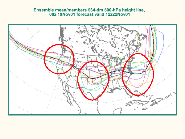
The post-processing produced the probability products that would become the public face of the ensemble. The first of these was the spaghetti plot: an isohypse contour at a chosen pressure level, drawn from each of the thirty-three members, overlaid on a single chart. Where the lines from the thirty-three members closely bunched, the forecast was confident. Where the lines spread out across the page, the forecast was uncertain. The spaghetti idiom – it had been used in research contexts before 1992 but became operational on 24 November of that year – gave forecasters a direct visual sense of where on the chart their confidence was high and where it was not.64 The second product was the probability map: the fraction of ensemble members exceeding a chosen threshold (a precipitation rate, a temperature, a windstorm strength) at each grid point. By colouring the map according to the probability, ECMWF produced fields that explicitly communicated the per-grid-point probability of a meteorological event.
The launch was not a spectacle. There was no press release, no headline in the Meteorological Magazine or the Bulletin of the American Meteorological Society, no celebratory event at Reading. The ECMWF Newsletter of winter 1992/93 covered the EPS launch with a technical article describing the system; it did not declare a new era.65 The Council had been briefed in advance; the national meteorological services had been notified; the documentation had been distributed. Tim Palmer would later recall in the EPS 20-years retrospective that ECMWF management had worried for years that the EPS was an expensive distraction from the deterministic forecast, and that the launch felt to him at the time more like an institutional probationary moment than a triumph.66 The case for ensembles among operational forecasters would have to be made afterwards, member-by-member, storm-by-storm, year-by-year, through the rest of the 1990s.
The case was made fastest by storms. The Burns Day storm of 25 January 1990 had already damaged the Met Office’s institutional credibility by being underforecast in the deterministic Bracknell system, and had reinforced the political case for probabilistic guidance.67 More dramatically, the Lothar and Martin windstorms that crossed France on 26 and 28 December 1999 would, seven years after the EPS launch, demonstrate the technique’s value in unambiguous terms.68 The deterministic forecasts at ECMWF, the Met Office, and Meteo-France had all suppressed the rapid deepening of Lothar over the Bay of Biscay; the EPS, by contrast, had given a clear probabilistic signal of a strong windstorm thirty-six to forty-eight hours ahead, with several ensemble members showing the explosive deepening that the deterministic forecast missed. The post-mortem reports on Lothar and Martin, published in 2000 and 2001, became the canonical demonstration of the EPS’s operational value. By 2002 the operational case had been won; the EPS was, across European meteorology, an accepted and used product.
By December 1996, four years after launch, the EPS was upgraded to fifty-one members with a resolution increase to TL159L31 (about 120 km grid spacing, 31 levels).69 The fifty-one-member configuration – one control plus twenty-five pairs of positive-negative singular-vector perturbations – would remain the operational standard for the next thirty years, surviving subsequent resolution increases to TL255L40 in November 2000, TL399L62 in February 2006, TL639L62 in March 2008, and TCo639L91 in March 2016. The membership of fifty-one was determined empirically as the sweet spot between the marginal probabilistic-score improvement of additional members (which tailed off above about forty members) and the additional computational cost.70 Daily production from 1 May 1994, twice-daily from 2004, the introduction of stochastic physics (SPPT in 1999, SKEB in 2009), and the Ensemble of Data Assimilations from June 2010 would all follow. None of those upgrades had been announced on 24 November 1992. They were the consequence of the system having simply worked, on its first operational day, exactly as designed.
6. NCEP and bred vectors
On Monday 7 December 1992, thirteen days after Palmer’s EPS had launched at Reading, the National Meteorological Center at Camp Springs in Maryland began operational ensemble prediction with a different method, on different hardware, with a different team.71 The institutional name “NCEP” – National Centers for Environmental Prediction – did not yet exist on that date. NMC would not be renamed NCEP until 1 October 1995, when as part of a NOAA National Weather Service reorganisation the Development Division of NMC became the Environmental Modeling Center (EMC) and the wider centre took the NCEP name.72 In December 1992 it was still NMC, and the Toth-Kalnay paper documenting the launch – published a few months later in the Bulletin of the American Meteorological Society – was therefore titled “Ensemble Forecasting at NMC: The Generation of Perturbations.”
The team had a different composition. Eugenia Kalnay, born 1 October 1942 in Buenos Aires, had taken the first woman’s PhD in meteorology at MIT in 1971 under Jule Charney.73 She had been the first woman faculty member in the MIT Department of Meteorology, had moved in 1979 to the Goddard Space Flight Center at NASA, had built up the Global Modeling and Simulation Branch there through the early 1980s, and in 1987 had taken over the Development Division at NMC under the chief scientist arrangements then in place. Her tenure at NMC from 1987 to 1997 – ten years – would see the launch of the bred-vector ensemble in December 1992, the operational deployment of the Spectral Statistical Interpolation (SSI) 3D-Var system on 25 June 1991 (a year and a half before the ensemble launch), the rollout of the NCEP/NCAR Reanalysis in 1996, and the renaming of the division to EMC in October 1995.
Working with her on the ensemble launch was Zoltan Toth, a Hungarian meteorologist of post-Communist generation who had arrived at NMC around 1990 – the exact year is not pinned down in available sources.74 Toth had trained in Hungary, had been mobile in the immediate post-1989 period when scientific cooperation with the United States became newly feasible, and had been recruited by Kalnay specifically for the ensemble-forecasting project. He was perhaps thirty years old when he arrived at Maryland; he would remain at NMC and then NCEP through the 1990s and 2000s, and is in 2026 a Senior Scientist at the Global Systems Laboratory of NOAA’s Earth System Research Laboratory in Boulder.
The third name on the canonical citation list is M. Steven Tracton, an operational scientist at NMC who handled the practical integration of the new ensemble products into the forecast floor. The Tracton and Kalnay 1993 Weather and Forecasting paper “Operational ensemble prediction at the National Meteorological Center: Practical aspects” is the operational complement to the Toth-Kalnay 1993 BAMS theoretical paper on perturbation generation.75 Tracton’s role was the institutional bridge between the research code that produced the bred vectors and the operational forecast desk that had to consume them.
The method these three deployed was the breeding of growing modes (BGM), or bred vector, technique.76 The procedure was conceptually simple. At each analysis cycle (typically 00 UTC at the time of the 1992 launch), a small random perturbation $\delta \mathbf{X}_0$ was added to the analysis $\mathbf{X}^{\text{anal}}_0$, forming a perturbed initial condition. Both the unperturbed control and the perturbed initial condition were integrated forward for one breeding cycle – 24 hours in the original 1992 system. The difference $\delta \mathbf{X}_1 = \mathbf{X}^{\text{pert}}_1 - \mathbf{X}^{\text{ctrl}}_1$ was computed at the end of the cycle and rescaled back to the original amplitude:
\[\delta \mathbf{X}'_1 = \delta \mathbf{X}_0 \cdot \frac{\|\delta \mathbf{X}_0\|}{\|\delta \mathbf{X}_1\|}\]The rescaled perturbation was added to the new analysis $\mathbf{X}^{\text{anal}}_1$ to form the bred initial condition for the next day. The process repeated indefinitely.
After many cycles, the rescaled perturbation $\delta \mathbf{X}’_n$ converged to a structure that grew, on average, at the rate of the dominant Lyapunov vector of the nonlinear model integrated through the analysis cycle. The convergence was the standard convergence of the power method for estimating the leading eigenvector of a matrix: repeated application of the operator to a starting vector, with rescaling, asymptotes to the eigenvector of largest eigenvalue. The bred vector was, in the asymptotic limit, a flow-dependent estimate of the leading Lyapunov vector of the operational analysis-forecast cycle.
The conceptual analogy that helps: bred vectors are what you would get if you took a perturbation at the start of the operational cycle, let the nonlinear model do whatever it wanted to it for a day, and then scaled it back down at the end. After many cycles, the perturbation has “learned” what kinds of structures the model amplifies – because the structures that the model damps have been progressively scaled down out of contention, while the structures that the model amplifies have been preserved through the rescaling. The asymptotic bred vector is the structure that the operational system itself most readily amplifies.
The advantages of breeding over singular vectors were operational. No adjoint model was required. Breeding used only the nonlinear forecast model, run twice (control plus perturbed) per breeding cycle per bred direction. NMC in 1992 did not have a tangent-linear and adjoint of the operational MRF model; it did not have 4D-Var; it could not have implemented singular-vector ensembles even if it had wanted to. The breeding method’s hardware demand was modest: roughly two extra forecast integrations per cycle per bred-vector pair – an order of magnitude cheaper than the Lanczos iteration on tangent-adjoint pairs that ECMWF was running. For Kalnay’s team in 1991-92, breeding was the only operationally feasible perturbation method on the Cray C90 that NMC had then in operation.77
The disadvantages were intellectual. Bred vectors were not optimal in any well-defined sense: they were not the directions of fastest growth over any particular time. They were not metric-independent in any deep way; the rescaling norm did affect the asymptotic structure, although the dependence was weaker than the singular-vector metric dependence. They converged to the dominant Lyapunov vector, but the Oseledec convergence to the asymptotic Lyapunov vector is a finite-time statement only up to second-order corrections, and for the 1-day breeding cycle the bred vectors were a noisy estimate of the Lyapunov vector. None of these intellectual concerns turned out to matter much in practice: bred vectors produced ensembles with reasonable spread and reasonable probabilistic skill, on a computing budget that NMC could afford.
The 7 December 1992 configuration was: T62L18 model resolution (about 210 km grid spacing, 18 vertical levels), the MRF (Medium-Range Forecast) global model in spectral primitive-equation form, fourteen forecasts per day verifying on days 1 through 10 (including a control plus two pairs of bred perturbations at 00 UTC, supplemented by lagged-average forecasts from earlier cycles), 24-hour breeding cycle with rescaling at each analysis time, and 12-day forecast range.78 The configuration was deliberately lighter than ECMWF’s: fewer members, lower resolution, slightly shorter forecast, but daily rather than three-times-a-week production. By March 1994 the bred-vector ensemble was expanded on the Cray C90 to seven independent breeding cycles producing seventeen forecasts per day (one control plus ten perturbed at 00 UTC, plus four perturbed at 12 UTC, plus carry-over members), with the forecast extended to sixteen days. The 1994 expansion brought NMC into rough parity with the operational ECMWF EPS, with very different methods.79
The 1990s and early 2000s saw the bred-vector method evolve. In May 2006 NCEP replaced the original breeding cycle with the Ensemble Transform with Rescaling (ETR) method, due to Wei, Toth, Wobus, Zhu, and Kalnay 2008.80 ETR generalised breeding by jointly rescaling all the perturbations so that their covariance matched a target – typically derived from analysis-error estimates – rather than independently scaling each breeding cycle. The ETR method was closer to an ensemble Kalman filter approximation than to pure breeding; it represented the gradual convergence of the American operational ensemble lineage toward the EnKF framework that the Canadian Meteorological Centre had pioneered. By the GEFSv12 of 2020, the operational NCEP Global Ensemble Forecast System used a 31-member ensemble at C384 resolution (about 25 km grid spacing) on the FV3-based GFS, with stochastic physics, four cycles a day, sixteen-day forecasts – and an initial-perturbation method that, while descended from breeding, had been substantially modified through twenty-eight years of operational experience.
The institutional context for the December 1992 launch deserves a closer look. NCEP/EMC was, in 1992, a smaller operation than ECMWF: perhaps fifteen scientists in the Development Division compared with ECMWF’s research department of forty or fifty. Kalnay’s directorship was the first woman’s directorship of the centre and would remain a remarked-upon fact through her tenure. The 1992 EMC also had to handle, beyond the ensemble launch, the simultaneous rollout of the Spectral Statistical Interpolation 3D-Var system that John Derber and David Parrish had brought operational on 25 June 1991 – the world’s first operational 3D-Var.81 The combined SSI + bred-vector ensemble made NCEP, in 1992, the most analytically ambitious operational shop in the world by a small margin – ECMWF would catch up with 3D-Var operational in early 1996 and 4D-Var on 25 November 1997. The institutional self-description on the EMC website would later describe these as the “first operational ensemble forecasting, first operational 3D-Var” of the centre’s history.82 The institutional self-description is mildly contested by the European centre, but the spirit is right: NCEP’s 1992 was a remarkable operational year.
The thirteen-day gap between ECMWF’s 24 November and NCEP’s 7 December was, as noted in the cold open, not coordinated. The two centres had been working in parallel on overlapping but distinct technical agendas for several years. Kalnay and Palmer were in contact through the AMS annual meetings and through the international predictability research community; they were not coordinating launches. The fact that the two operational ensemble systems crossed the operational threshold within two weeks of each other in late 1992 is an artefact of two centres reaching operational readiness at roughly the same time, with different methods, in the same intellectual moment.
The intellectual moment was Lorenz’s.
7. The Lorenz connection
Edward Norton Lorenz had been born in West Hartford, Connecticut on 23 May 1917 and was, in late 1992, seventy-five years old.83 He had been at MIT since 1948, where he had spent his entire career as a member of the Department of Meteorology – later the Department of Earth, Atmospheric, and Planetary Sciences after the 1983 reorganisation that Post 41 of this series covered in detail.84 His 1963 paper “Deterministic non-periodic flow” in the Journal of the Atmospheric Sciences had been the foundational text of chaos theory and was, in late 1992, twenty-nine years old. His 1969 paper “The predictability of a flow which possesses many scales of motion” in Tellus had been the foundational text of medium-range predictability research and was, in late 1992, twenty-three years old.
The intellectual debt of both 1992 launches to Lorenz is documented in their primary citations. Palmer-Molteni-Mureau-Buizza-Chapelet-Tribbia 1992 (ECMWF Technical Memorandum No. 188), the EPS proposal, opened with the predictability-as-flow-dependent argument that comes directly out of Lorenz 1969.85 Molteni-Buizza-Palmer-Petroliagis 1996 in QJRMS would extend the same citation. Toth-Kalnay 1993 BAMS opened with a paragraph crediting Lorenz 1963 and 1969 for establishing “a deterministic prediction system has limited predictability” and arguing for ensemble averaging as a consequence. Both papers also cited Lorenz 1965 in Tellus – the lesser-known paper, “A study of the predictability of a 28-variable atmospheric model,” that Palmer would later credit in his 2019 retrospective as the first appearance of singular value decomposition in a meteorological context.86
There is no surviving public record of Lorenz being formally consulted on the design of either operational system. The ECMWF predictability division and Palmer’s group operated as Lorenz’s intellectual heirs without his direct involvement in their operational decisions. Kalnay had been at MIT through the early 1970s, had taken her PhD with Charney, and would have known Lorenz personally – they had been in the same department, and Lorenz was a senior figure when Kalnay was a graduate student. The MIT connection makes the NCEP bred-vector lineage a direct continuation of the dynamical-systems formalism that Lorenz had championed at MIT through the 1960s and 1970s. Whether Lorenz commented on the 24 November 1992 or 7 December 1992 launches in 1992 itself is not documented; Palmer’s 2009 Royal Society biographical memoir of Lorenz describes Lorenz as “fascinated” by the operational success of ensemble forecasting but does not record a specific 1992 reaction.87
The first documented direct interaction came nearly three years after the launches, at the ECMWF Seminar on Predictability at Reading from 4 to 8 September 1995.88 The seminar was a week-long meeting of perhaps fifty researchers, the predictability research community taking stock three years into the operational ensemble era. Lorenz was the keynote speaker. His lecture title was “Predictability: A Problem Partly Solved,” and was a deliberate echo of the questions he had set in 1963 and 1969 – with the implicit observation that “partly” was the right qualifier.89 Ensemble forecasting had partly solved the problem he had set; it had not solved it completely.
The most consequential output of the 1995 seminar was a forty-equation toy model that Lorenz introduced for the first time at Reading. The Lorenz 96 model – forty grid points around a latitude circle, with each grid point’s tendency given by a small system of coupled nonlinear ODEs of the form
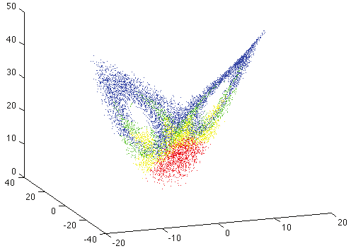
\[\frac{dX_i}{dt} = (X_{i+1} - X_{i-2}) X_{i-1} - X_i + F\]with $F = 8$ providing the forcing that made the system chaotic – was designed explicitly as a test bed for numerical weather prediction.90 The model was simple enough to integrate thousands of times in parametric studies, complex enough to capture the structural features of operational models, and small enough to allow exhaustive analysis of its invariant set. It would become, over the next thirty years, the canonical toy model on which ensemble methods, data assimilation algorithms, parameter estimation schemes, and predictability analyses are first tested before being deployed on full operational models. By 2026, the Lorenz 96 model has been the subject of perhaps five hundred academic papers and is taught in every graduate-level data assimilation course.
That Lorenz introduced the model at ECMWF, in September 1995, three years after the EPS had become operational, is a marker of his engagement with the operational ensemble community by mid-1995. The invitation to the seminar had almost certainly come from Palmer’s section. The fact that Lorenz had constructed a new toy model specifically aimed at NWP testing suggests prior dialogue between Palmer’s section and Lorenz, even if the pre-1995 documentation of that dialogue is thin. By 1995, certainly, Lorenz was a regular interlocutor of the operational ensemble community, and the Lorenz 96 model was the gift he gave them.
The intellectual debt that the 1992 ensembles owed to Lorenz can be summarised in three points. The first is the finite predictability horizon: Lorenz 1969 established, on the basis of upscale-cascade arguments in a $k^{-5/3}$ inertial-range spectrum, that the atmosphere has an intrinsic predictability horizon of order two weeks, and that this horizon is statistical rather than deterministic – some flows are much more predictable than others, and the right forecasting system needs to communicate the per-day, per-flow uncertainty.91 The 1992 ensembles were the operational implementation of that statement. The second is the non-modal growth of finite-time perturbations: Lorenz 1965 in the 28-variable model had computed, by what is functionally a singular value decomposition of the propagator, that the growth rates of initial errors varied with the synoptic flow regime from a few days to a few weeks.92 This empirical seed of flow-dependent predictability became the singular-vector framework that Palmer’s group would operationalise. The third is the probabilistic reframing of weather forecasting itself: Lorenz had argued throughout his career that the right unit of analysis was the probability distribution, not the deterministic trajectory, and that the skill of a forecast was best measured by reliability and resolution scores rather than by RMS errors of point estimates.93 The 1992 ensembles instantiated this reframing operationally.
Lorenz would attend the 2002 anniversary symposium for the EPS at Reading and would, by all accounts, be pleased.94 He would die in Cambridge, Massachusetts on 16 April 2008, eighty-nine years old, having lived to see his intellectual descendants populate every major operational forecasting centre on Earth.95 His 1996 Reading lecture proceedings, “Predictability: A Problem Partly Solved,” remain in print as one of the most-cited single chapters in the history of dynamical meteorology, and the Lorenz 96 model that he introduced there continues to anchor the methodological development of ensemble forecasting in 2026 just as it did in the late 1990s.
8. Evolution to 2026
The thirty-four years between 24 November 1992 and 20 May 2026 saw the ensemble principle generalised, extended, and absorbed into every layer of the operational forecasting stack. Six developments stand out.
The first was the fifty-one-member EPS upgrade of December 1996.96 ECMWF moved from the 33-member T63L19 launch configuration to 51 members at TL159L31 (about 120 km grid spacing, 31 vertical levels), one control plus 25 pairs of singular-vector perturbations. The fifty-one-member figure was determined empirically and would prove unusually durable, surviving every subsequent resolution increase. Daily production began on 1 May 1994 (still at 33 members, T63L19); twice-daily production began in 2004 at the higher resolution. The pattern of resolution increases – roughly every five years, tied to supercomputer upgrades from the Cray C90 through Fujitsu VPP, IBM Power, Atos BullSequana, and the modern HPE Cray EX – pushed the ensemble from T63 (210 km) in 1992 to TL159 (120 km) in 1996, TL255 (80 km) in 2000, TL399 (50 km) in 2006, T639 (32 km) in 2008, and TCo639 (18 km) in March 2016, where it has remained.97
The second was stochastic physics, introduced through Buizza, Miller, and Palmer 1999 in QJRMS.98 The 1999 paper acknowledged that initial-condition perturbations alone produced under-dispersive ensembles in the medium range – by day seven the ensemble spread was smaller than the ensemble-mean RMS error – and proposed that the missing dispersion came from neglected model error. The fix was the Stochastically Perturbed Parametrization Tendencies (SPPT) scheme: the total physics tendency on the right-hand side of each prognostic equation, summing radiation, convection, boundary layer, gravity waves, and clouds, was multiplied by $1 + r(\mathbf{x}, t)$ where $r$ was a smoothly-varying random field with zero mean and prescribed variance. The amplitude was tuned to represent the uncertainty in the total parametrised tendency. SPPT became operational at ECMWF in late 1999 and was adopted by every major centre over the following decade. A second scheme, Stochastic Kinetic Energy Backscatter (SKEB), due to Glenn Shutts at the Met Office, would represent the upscale energy transfer that grid-scale damping removed; SKEB became operational at ECMWF in 2009.99 The combination of SV initial perturbations + SPPT + SKEB was the operational EPS recipe through the 2010s.
The third was the ensemble Kalman filter lineage, separate from but complementary to the SV-versus-breeding divide. The EnKF, developed in the 1990s by Geir Evensen at the Nansen Center in Bergen and refined through Burgers, van Leeuwen, and Evensen 1998 and Houtekamer and Mitchell 1998, used an ensemble of model integrations to estimate the flow-dependent background-error covariance, then applied a Kalman-filter-style update at each observation time.100 The end-of-cycle ensemble was the natural initial set for an ensemble forecast: no separate SV or bred-vector calculation needed. The Canadian Meteorological Centre put the world’s first operational EnKF into routine production on 12 January 2005, providing the initial conditions for the Canadian medium-range ensemble.101 The CMC deployment opened a third lineage of operational ensembles: ECMWF SV-based, NCEP breeding-based, CMC EnKF-based, all running in parallel through the 2010s, with TIGGE multi-model studies showing that each captured something the others did not.
The fourth was the Ensemble of Data Assimilations (EDA) at ECMWF, operational from June 2010.102 EDA was a separate ensemble of 4D-Var analyses, each driven by perturbed observations and perturbed background fields. The EDA produced a sample of analyses whose spread estimated the flow-dependent analysis-error covariance. The EDA outputs were used in two ways: as initial perturbations in the EPS, additively combined with the SVs (so that the modern ENS used both EDA and SV perturbations as complementary sources of initial spread), and as the flow-dependent background-error covariance for the deterministic 4D-Var, in the hybrid 4DEnVar scheme that blended ensemble and climatological covariances. The hybrid 4DEnVar approach – a combination of variational assimilation with flow-dependent ensemble-derived background-error covariances – became the operational standard at every major centre by the mid-2010s. The 1992 divide between SV and breeding had been subsumed into a unified ensemble-variational framework.
The fifth was TIGGE, the THORPEX Interactive Grand Global Ensemble archive that launched at ECMWF in October 2006 as part of the WMO THORPEX programme.103 TIGGE archived ensemble forecasts from ten global centres (ECMWF, JMA, Met Office, CMA, NCEP, MSC, Meteo-France, BOM, CPTEC, KMA) at 6-hourly resolution for a wide range of surface and pressure-level variables, with a 48-hour delay before public release. By the late 2000s TIGGE had enabled the first systematic multi-centre, multi-model ensemble research at operational lead times, demonstrating that multi-model ensembles routinely outperform any single-model ensemble for medium-range probabilistic forecasts.104 The TIGGE archive is hosted at ECMWF and at CMA and remains the standard verification testbed for operational ensemble research in 2026. The S2S Prediction Project, launched as a joint WMO/WWRP project in 2013, extended the TIGGE archive concept into the 11- to 60-day subseasonal range.105 S2S models couple to interactive oceans, have larger ensembles, and target lead times where neither pure-atmosphere medium-range forecasts nor pure-coupled seasonal forecasts had previously provided guidance.
The sixth was the rise of machine-learning weather models in the 2020s, which deserves its own treatment but bears mentioning here because of its connection to the ensemble framework. By 2024-2025 the operational forecasting landscape had been disrupted by ML-trained surrogate models – GraphCast at DeepMind, Pangu-Weather at Huawei, FourCastNet at NVIDIA, GenCast at DeepMind for probabilistic forecasts – that produced ten-day forecasts at competitive skill to ECMWF’s deterministic HRES at one-thousandth the computational cost.106 Palmer himself, in his retirement-era writings of 2023-2025, has been an enthusiastic engager with the ML developments, viewing them as one more confirmation that the right way to think about weather forecasting is statistical: the ML models are, in effect, learned surrogates for the propagator that the singular-vector EPS uses, and the same probabilistic reasoning applies.107 The ML era is in 2026 still very young, and how ML ensembles will reshape the operational landscape is not yet clear; what is clear is that the conceptual framework Palmer established in 1992 – ensemble forecasting as the operational answer to chaos – remains the framework within which ML systems are being deployed and evaluated.
By 2026 the operational ensemble configuration at ECMWF is 51 members at TCo639L91 (cubic-octahedral reduced Gaussian grid at about 18 km grid spacing, 91 vertical levels) for the first 15 days, then TCo319L91 (about 36 km) extending to day 46 – the extended-range monthly forecast, merged into the EPS production in 2008 – with SPPT, SKEB, EDA initial perturbations supplemented by singular vectors over different regions, and the modern hybrid 4DEnVar driving the deterministic 4D-Var.108 The ENS resolution has been TCo639L91 since 8 March 2016; the deterministic HRES has been TCo1279L137 since June 2016. The unified deterministic-ensemble configuration that ECMWF announced for the late 2020s – a single resolution for HRES and ENS, abolishing the historical asymmetry where the ensemble ran coarser than the deterministic – is the next planned structural shift.
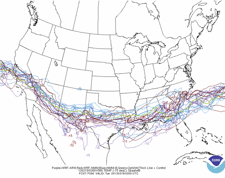
NCEP in 2026 runs GEFSv12 at C384 resolution (about 25 km) on the FV3-based GFS, with 31 members, four cycles a day, sixteen-day forecasts, stochastic physics, and an initial-perturbation method that has evolved from breeding through ETR and is now closer to the EnKF lineage.109 The Canadian system uses a 256-member EnKF that traces back to the 12 January 2005 deployment. The Met Office runs MOGREPS, a 36-member ensemble at N640 resolution on the Unified Model, with stochastic physics and the Met Office hybrid 4D-Var. The UKMO, JMA, Meteo-France, DWD, BOM, CMA, and KMA all run ensembles, and the differences between them in any given week’s TIGGE archive are smaller than the differences between any single-centre’s deterministic and ensemble outputs. The ensemble principle is everywhere.
The conceptual closure of the 1992 launches is this. Lorenz had argued in 1969 that the atmosphere had a finite intrinsic predictability horizon. Palmer and Kalnay had built, in 1992, the operational machinery to push that horizon further by giving forecasters the per-day, per-flow uncertainty estimate that a single deterministic forecast could not provide. By 2026, thirty-four years on, the machinery has been generalised across every centre, every variable, every lead time from hours to seasons. The operational meteorologist of 2026 does not think of the EPS as a research-flavoured production stream that some forecasters consult and most do not; the operational meteorologist of 2026 thinks of the ensemble as the primary forecast, with the deterministic high-resolution forecast as one trajectory through it. The conceptual shift that Lorenz had argued for and that Palmer had operationalised on 24 November 1992 has become the operational default.
9. Palmer’s Oxford turn
Tim Palmer left ECMWF in 2010, with some institutional ambiguity about whether the actual move was in 2010 or 2011.110 The substantive event was his selection in 2010 as one of the Royal Society 350th Anniversary Research Professors – a set of new chairs the Royal Society had created to celebrate its 350th anniversary, awarded competitively across all sciences. Palmer’s chair, titled Royal Society Research Professor in Climate Physics, was based at Oxford University’s Department of Physics, in the Atmospheric, Oceanic and Planetary Physics sub-department, with the office on the second floor of the Robert Hooke Building. He also became a Professorial Fellow of Jesus College, Oxford, and from 2010 the Co-Director of the Oxford Martin Programme on Modelling and Predicting Climate at the Oxford Martin School. The 2010 announcement was the move; the 2011 figure that ECMWF’s Newsletter 134 author-bio cites may reflect a transitional period during which Palmer divided his time between Reading and Oxford during the academic year 2010-11. The substantive change of institutional affiliation was the 2010 Royal Society appointment.111
Palmer’s twenty-four years at ECMWF had produced, alongside the EPS, three major institutional projects that deserve mention. PROVOST (PRediction Of climate Variations On Seasonal to interannual Time-scales), an EU Framework 4 project that Palmer led from 1996, applied the ensemble methodology to seasonal prediction, particularly the El Nino-Southern Oscillation prediction problem.112 DEMETER (Development of a European Multimodel Ensemble system for seasonal to interannual prediction), an EU Framework 5 project that Palmer led from 2002, developed the multi-coupled-model ensemble approach that would become the methodological backbone of the IPCC Fourth Assessment Report’s seasonal-prediction assessments.113 And throughout the 2000s Palmer was a contributor to the IPCC, on every assessment report from FAR (1990) through AR6 (2021), and was one of the IPCC contributors who in 2007 shared in the Nobel Peace Prize awarded jointly to the IPCC and Al Gore.114
The Oxford period from 2010 to the present has been Palmer’s late-career intellectual integration. The Royal Society chair freed him from the operational responsibilities of the ECMWF directorate-level position and allowed him to write, lecture, and pursue research questions that lay across the boundaries of his fields. He served as President of the Royal Meteorological Society in 2011-2012. He maintained an honorary affiliation as an Inaugural Fellow of ECMWF. He took visiting positions at the University of Washington and at the Isaac Newton Institute in Cambridge, where he was Rothschild Distinguished Visiting Professor. In the mid-2010s his research interests began to include quantum-mechanical foundations: a deterministic, fractal-state-space account of quantum mechanics that he called the Cosmological Invariant Set Postulate. The Oxford Quantum Institute carries his affiliation. He became Emeritus at Oxford Physics in the early 2020s and is now Emeritus Fellow at Jesus College, but remains active in writing and speaking through 2026.
The integrative book of the late period is The Primacy of Doubt (Oxford University Press / Basic Books, 18 October 2022), Palmer’s accessible-to-the-general-reader treatment of his life’s work.115 The book’s subtitle, in the UK edition, is “From climate change to quantum physics, how the science of uncertainty can help us understand our chaotic world”; the US edition reverses the subtitle. The central argument is that uncertainty should be elevated “not as an afterthought, but as a matter of primal importance”; that climate action should be “framed in terms of risk” rather than certainty about catastrophic outcomes; and that chaotic systems are “predictable most of the time, but spectacularly unpredictable on occasion.” The book endorsements include Roger Penrose (“a remarkably broad-ranging account of uncertainty in physics, in all its various aspects – I strongly recommend this highly thought-provoking book”), Martin Rees, and Brian Clegg.116 The Primacy of Doubt is, in 2026, the most accessible single portal into Palmer’s worldview for a general reader.
The 2010s and 2020s brought a sequence of awards that consolidated Palmer’s standing as the institutional architect of operational ensemble forecasting. The AMS Carl-Gustaf Rossby Research Medal in 2010 cited his “fundamental contributions to understanding the role of nonlinear processes in the predictability of weather and climate.”117 The European Meteorological Society Silver Medal in 2012, presented at Lodz, Poland on 12 September 2012, recognised “his pioneering work on predictability of weather and climate and his outstanding skills and commitment in communicating the underlying concepts to non-specialists.”118 The Dirac Medal of the Institute of Physics in 2014 cited him for “development of probabilistic weather and climate prediction systems.” The CBE – Commander of the Order of the British Empire in the 2015 New Year Honours, for services to science – making him Professor Tim Palmer CBE FRS, not Sir Tim, despite the persistent confusion in some secondary sources.119 The EGU Lewis Fry Richardson Medal in 2018 cited his “fundamental contributions to the conception and practical implementation of a system for ensemble weather prediction.”120 The Royal Astronomical Society Gold Medal for Geophysics in 2023; the Royal Irish Academy Honorary Membership in 2023, drawing on his Irish-side maternal nationality; and most consequentially the WMO IMO Prize 2023, announced 6 June 2023, the World Meteorological Organization’s highest single honour, named after the International Meteorological Organization that preceded the WMO.121 Palmer follows Lorenz (2000) and Houghton (1998) on the IMO laureate list. The 2023 IMO Prize citation reads: “Ensemble prediction is almost universally used in weather prediction today, on all timescales. Developing reliable ensembles lies at the heart of many weather service strategic plans. Importantly it is completely transforming the way in which disaster relief agencies operate.”
The coda is institutional and personal at once. The Predictability and Diagnostics Division that Palmer headed at Reading from 1986 to 2002 was renamed the Probabilistic Forecasting and Diagnostics Division in 2002, reflecting the centrality of probabilistic seasonal forecasting that PROVOST and DEMETER had established. The division still exists at ECMWF in 2026, with leadership having passed through several Palmer successors including Martin Leutbecher. Roberto Buizza moved from ECMWF to the Sant’Anna School of Advanced Studies at Pisa and then to the University of Bologna in the mid-2010s, where he continues to publish on ensemble methods. Franco Molteni retired from ECMWF in the late 2010s and continues to consult. Eugenia Kalnay published her textbook Atmospheric Modeling, Data Assimilation and Predictability (Cambridge University Press, 2003), which has become the standard graduate-level reference for the field; she moved from NCEP/EMC to the University of Maryland in 1999, where she co-founded the Weather/Chaos Group with the mathematician James A. Yorke, and died on 13 August 2024 at age 81 in Maryland.122 Zoltan Toth remains active at NOAA’s Global Systems Laboratory in Boulder.
Palmer lives now in the West Berkshire Downs, the quiet rural area west of Reading that puts him within commute of both Oxford and ECMWF. He plays guitar in a band; his wife Gill’s much-repeated line on the band-mates is that they joke he is “desperately trying to save the planet – while living on another one.”123 He composes original poetry. He plays golf and mountain-bikes across the West Berkshire Downs. He continues to write and lecture, and the Primacy of Doubt paperback of 2024 along with the follow-on essays through 2025 and into 2026 have kept him visible in the public-intellectual phase of his career. In 2026 he is 73 years old.
Coda
The thirty-three forecasts that ran on the Cray Y-MP/8 at Shinfield Park on Tuesday 24 November 1992 were the operational implementation of a conceptual argument that Edward Lorenz had been making for thirty years. The fourteen forecasts that ran on the Cray C90 at Camp Springs on Monday 7 December 1992 were the same argument’s American implementation, by a different method, on a smaller machine, two weeks later. Together they were the operational answer to a question that had been on the table since the 1960s and unresolved through the 1970s and 1980s: how do you forecast an inherently chaotic system in a way that communicates per-day, per-flow uncertainty to the people who have to make decisions based on the forecast?
The answer was the ensemble. Thirty-three lines on the map, drawn from thirty-three forecasts starting from thirty-three different initial states, gave the European forecaster of late November 1992 the first operationally available probabilistic medium-range product. Fourteen lines on the map, drawn from fourteen forecasts starting from fourteen bred-vector initial states, gave the American forecaster of early December 1992 the same product by a different recipe. The two ensemble systems would converge through the 2000s and 2010s into a hybrid framework; the conceptual breakthrough was the move from one line to many.
What the move enabled was a different way of using a forecast. The deterministic single forecast had been the operational product of weather forecasting since the ENIAC integration of March 1950 and remained so through the 1970s and 1980s; the user of the forecast had to make their own implicit estimate of how reliable the forecast was on any given day. The ensemble product made that estimate explicit. A user could read off the page how confident the forecasting centre was, on any given day, in its prediction of the high over the Bay of Biscay or the low over the Baltic. They could plan their hedges against the alternative possibilities the ensemble was showing. They could allocate emergency-services attention in proportion to the probability of severe weather. They could, in short, treat the forecast as a probability distribution rather than as a point estimate, which is what every operational use of a chaotic forecast really requires.
The ensemble principle is now universal. Hurricane track cones are ensembles. Climate projections are ensembles. Air-quality forecasts are ensembles. Pandemic projections in 2020 and 2021 were ensembles. Subseasonal-to-seasonal forecasts for energy traders, agricultural insurers, and reinsurance underwriters are ensembles. The conceptual move that Palmer’s team made at Reading on 24 November 1992 – the move from “what will the weather do” to “what is the probability distribution over what the weather might do” – has been generalised across nearly every domain in which long-range physical prediction matters. The thirty-three lines on the map of 24 November 1992 are the ancestor of all of it.
Tim Palmer would write in his 2019 retrospective that “forecasting within this so-called deterministic limit of predictability has become inherently probabilistic.”124 He meant: within the two-week horizon Lorenz had identified in 1969, the right forecast is a probability distribution, not a trajectory. The 24 November 1992 launch of the ECMWF EPS was the day that statement stopped being a theoretical claim and started being an operational fact. Everything in operational meteorology since then has been the working out of its consequences.
The intellectual genealogy of the launch closes with three names. Edward Lorenz at MIT had argued for the conceptual move in 1963, 1965, and 1969, and was three years from delivering the Lorenz 96 model at the 1995 ECMWF Seminar on Predictability when the launch happened. Eugenia Kalnay at NCEP/EMC had carried the MIT-Charney intellectual lineage into the American operational ensemble, and would launch the bred-vector ensemble thirteen days after Palmer. Tim Palmer at ECMWF had carried the Sciama-Hut general-relativity instincts – the willingness to take a finite-dimensional dynamical-systems view of an infinite-dimensional system – into the European operational ensemble, and had built the institutional and computational infrastructure that put the singular-vector EPS into production on 24 November 1992. The three names are the spine of the story. The thirty-three forecasts were the result.
Footnotes
Sources
Primary papers
- Lorenz, E. N., 1963: “Deterministic non-periodic flow,” J. Atmos. Sci. 20, 130-141.
- Lorenz, E. N., 1965: “A study of the predictability of a 28-variable atmospheric model,” Tellus 17, 321-333.
- Lorenz, E. N., 1969: “The predictability of a flow which possesses many scales of motion,” Tellus 21, 289-307.
- Lorenz, E. N., 1996: “Predictability: A problem partly solved,” in Proceedings of the ECMWF Seminar on Predictability, Reading, 4-8 September 1995, ECMWF.
- Hoffman, R. N., and Kalnay, E., 1983: “Lagged average forecasting, an alternative to Monte Carlo forecasting,” Tellus A 35, 100-118.
- McIntyre, M. E., and Palmer, T. N., 1983: “Breaking planetary waves in the stratosphere,” Nature 305, 593-600.
- Brankovic, C., Palmer, T. N., Molteni, F., Tibaldi, S., and Cubasch, U., 1990: “Extended-range predictions with ECMWF models: time-lagged ensemble forecasting,” QJRMS 116, 867-912.
- Palmer, T. N., Molteni, F., Mureau, R., Buizza, R., Chapelet, P., and Tribbia, J., 1992: “Ensemble prediction,” ECMWF Tech. Memo. No. 188.
- Mureau, R., Molteni, F., and Palmer, T. N., 1993: “Ensemble prediction using dynamically conditioned perturbations,” QJRMS 119, 299-323.
- Toth, Z., and Kalnay, E., 1993: “Ensemble forecasting at NMC: The generation of perturbations,” Bull. Amer. Meteor. Soc. 74, 2317-2330.
- Tracton, M. S., and Kalnay, E., 1993: “Operational ensemble prediction at the National Meteorological Center: Practical aspects,” Wea. Forecasting 8, 379-398.
- Palmer, T. N., and Molteni, F., 1993: “On the dynamics of large extra-tropical-circulation anomalies,” QJRMS 119, 269-298.
- Buizza, R., and Palmer, T. N., 1995: “The singular vector structure of the atmospheric global circulation,” J. Atmos. Sci. 52, 1434-1456.
- Molteni, F., Buizza, R., Palmer, T. N., and Petroliagis, T., 1996: “The ECMWF Ensemble Prediction System: Methodology and validation,” QJRMS 122, 73-119.
- Toth, Z., and Kalnay, E., 1997: “Ensemble forecasting at NCEP and the breeding method,” Mon. Wea. Rev. 125, 3297-3319.
- Palmer, T. N., Gelaro, R., Barkmeijer, J., and Buizza, R., 1998: “Singular vectors, metrics, and adaptive observations,” J. Atmos. Sci. 55, 633-653.
- Buizza, R., Miller, M., and Palmer, T. N., 1999: “Stochastic simulation of model uncertainties in the ECMWF Ensemble Prediction System,” QJRMS 125, 2887-2908.
Retrospectives
- Palmer, T. N., 2019: “The ECMWF ensemble prediction system: Looking back (more than) 25 years and projecting forward 25 years,” QJRMS 145 (S1), 12-24. arXiv:1803.06940.
- Barkmeijer, J., Buizza, R., Kallen, E., Molteni, F., Mureau, R., Palmer, T. N., Tibaldi, S., Tribbia, J., 2012/13: “20 years of ensemble prediction at ECMWF,” ECMWF Newsletter 134, pp. 16-32. DOI 10.21957/l6nteidw.
- Buizza, R., and Richardson, D., 2017: “25 years of ensemble forecasting at ECMWF,” ECMWF Newsletter 153 (Autumn 2017).
Books
- Kalnay, E., 2003: Atmospheric Modeling, Data Assimilation and Predictability. Cambridge University Press.
- Palmer, T. N., and Hagedorn, R., eds., 2006: Predictability of Weather and Climate. Cambridge University Press.
- Palmer, T. N., 2022: The Primacy of Doubt. Oxford University Press / Basic Books.
Institutional sources
- ECMWF, “History,” https://www.ecmwf.int/en/about/who-we-are/history.
- ECMWF, “Tim Palmer Festschrift,” https://www.ecmwf.int/en/about/media-centre/media-resources/tim-palmer-festschrift/.
- NCEP/EMC, “Ensemble Background,” https://www.emc.ncep.noaa.gov/gmb/ens/info/ens_detbak.html.
- WMO, “Prof. Timothy Palmer named IMO Prize laureate,” 6 June 2023, https://wmo.int/media/news/prof-timothy-palmer-named-imo-prize-laureate.
Encyclopedia entries
- Wikipedia, “Tim Palmer (physicist),” https://en.wikipedia.org/wiki/Tim_Palmer_(physicist).
- Wikipedia, “Eugenia Kalnay,” https://en.wikipedia.org/wiki/Eugenia_Kalnay.
- Wikipedia, “Lennart Bengtsson,” https://en.wikipedia.org/wiki/Lennart_Bengtsson.
Cross-linked posts in this series
- Post 41, “The Coyote Who Found Chaos” (Lorenz): /weather/hpc/history/2026/05/15/The-coyote-who-found-chaos.html
- Post 42, “The First in Bracknell” (Met Office Cyber 205): /weather/hpc/history/2026/05/15/The-first-in-Bracknell.html
- Post 43, “The Package Deal” (Phillips): /weather/hpc/history/2026/05/17/The-package-deal.html
- Post 44, “The Book That Crossed the Iron Curtain” (Gandin/OI): /weather/hpc/history/2026/05/17/The-book-that-crossed-the-curtain.html
- Post 35, “A Billion Butterflies” (Shukla): /weather/hpc/history/2026/05/10/A-billion-butterflies.html
- Post 34, “First Cray in Europe” (ECMWF founding): /weather/hpc/history/2026/05/09/First-Cray-in-Europe.html
-
ECMWF, “History,” https://www.ecmwf.int/en/about/who-we-are/history. The page states unambiguously: “The first ensemble predictions, produced as part of the operational forecasting system, were achieved on 24 November 1992.” Also: Barkmeijer, J., Buizza, R., Kallen, E., Molteni, F., Mureau, R., Palmer, T. N., Tibaldi, S., Tribbia, J., 2012/13: “20 years of ensemble prediction at ECMWF,” ECMWF Newsletter 134 (Winter 2012/13), pp. 16-32. DOI 10.21957/l6nteidw. https://www.ecmwf.int/sites/default/files/elibrary/2013/17373-20-years-ensemble-prediction-ecmwf.pdf. Newsletter 134 verbatim: “Twenty years ago, on 24 November 1992, the first ensemble forecasts were produced at ECMWF.” Newsletter 153 of 2017 contains a typo giving 19 December 1992; the canonical date is 24 November. ↩
-
Toth, Z., and Kalnay, E., 1993: “Ensemble forecasting at NMC: The generation of perturbations,” Bull. Amer. Meteor. Soc. 74, 2317-2330. https://journals.ametsoc.org/view/journals/bams/74/12/1520-0477_1993_074_2317_efantg_2_0_co_2.xml. The 7 December 1992 launch date is also confirmed in the NCEP EMC Ensemble Background page at https://www.emc.ncep.noaa.gov/gmb/ens/info/ens_detbak.html. ↩
-
Edward Norton Lorenz was born 23 May 1917 in West Hartford, Connecticut. Emanuel, K., 2011: “Edward Norton Lorenz,” NAS Biographical Memoirs. http://www.nasonline.org/publications/biographical-memoirs/memoir-pdfs/lorenz-edward.pdf. ↩
-
Lorenz, E. N., 1969: “The predictability of a flow which possesses many scales of motion,” Tellus 21, 289-307. https://onlinelibrary.wiley.com/doi/abs/10.3402/tellusa.v21i3.10086. ↩
-
Palmer was awarded the CBE in the 2015 New Year Honours for services to science. He is “Professor Tim Palmer CBE FRS,” not “Sir Tim Palmer” – the persistent confusion with a knighthood in some secondary sources is incorrect. Wikipedia, “Tim Palmer (physicist),” https://en.wikipedia.org/wiki/Tim_Palmer_(physicist). His birth date (31 December 1952, Kingston upon Thames) and Bristol-Oxford-Met-Office-ECMWF chronology are documented in the same source. ↩
-
The five-person core team is documented in Newsletter 134, ECMWF Festschrift web pages (https://www.ecmwf.int/en/about/media-centre/media-resources/tim-palmer-festschrift/), and Palmer 2019. Mureau’s role on the operational-model singular-vector testing is in Mureau, R., Molteni, F., and Palmer, T. N., 1993: “Ensemble prediction using dynamically conditioned perturbations,” QJRMS 119, 299-323. Tribbia’s NCAR detail and IFS adjoint work is described in Palmer 2019 (arXiv:1803.06940) and Newsletter 134. ↩
-
Eugenia Kalnay was Director of NCEP/EMC from 1987 to 1997, the first woman to hold the position. Wikipedia, “Eugenia Kalnay,” https://en.wikipedia.org/wiki/Eugenia_Kalnay. Born 1 October 1942 in Buenos Aires, died 13 August 2024 in Maryland aged 81. ↩
-
Toth, Z., and Kalnay, E., 1993: “Ensemble forecasting at NMC: The generation of perturbations,” Bull. Amer. Meteor. Soc. 74, 2317-2330. Tracton, M. S., and Kalnay, E., 1993: “Operational ensemble prediction at the National Meteorological Center: Practical aspects,” Wea. Forecasting 8, 379-398. ↩
-
ECMWF acquired its Cray Y-MP/8 in late 1989, with eight processors and a peak performance of about 2.4 GFLOPS, replacing the Cray X-MP/22 (two processors, peak around 470 MFLOPS) that had been the workhorse since 1986. The Cray C90 was installed at ECMWF in 1993, after the 24 November 1992 EPS launch ran on the Y-MP. Cray specifications: https://en.wikipedia.org/wiki/Cray_Y-MP. ↩
-
The 33-member configuration is documented in Palmer, T. N., Molteni, F., Mureau, R., Buizza, R., Chapelet, P., and Tribbia, J., 1992: “Ensemble prediction,” ECMWF Tech. Memo. No. 188; and in Molteni, F., Buizza, R., Palmer, T. N., and Petroliagis, T., 1996: “The ECMWF Ensemble Prediction System: Methodology and validation,” QJRMS 122, 73-119. Composition: 1 control + 16 positive perturbations + 16 negative perturbations along the 16 leading initial-time singular vectors. ↩
-
T63 spectral truncation corresponds to a roughly 1.875-degree gridpoint spacing, about 210 km at the equator. T63L19 – 63 zonal wavenumbers, 19 vertical levels – was the operational EPS resolution at ECMWF in late 1992; the deterministic forecast itself was running at T106L19 (about 125 km). ↩
-
Three-times-a-week production – Friday, Saturday, Sunday at 12 UTC – documented in Newsletter 134. Daily production began on 1 May 1994; twice-daily (00 and 12 UTC) from 2004. ↩
-
The 48-hour optimisation window is documented in Palmer, T. N., and Molteni, F., 1993: “On the dynamics of large extra-tropical-circulation anomalies,” QJRMS 119, 269-298; and Buizza, R., and Palmer, T. N., 1995: “The singular vector structure of the atmospheric global circulation,” J. Atmos. Sci. 52, 1434-1456. ↩
-
The total-energy norm is the kinetic-energy density plus the available-potential-energy density, integrated over the global atmosphere. Palmer, T. N., Gelaro, R., Barkmeijer, J., and Buizza, R., 1998: “Singular vectors, metrics, and adaptive observations,” J. Atmos. Sci. 55, 633-653. ↩
-
Lothar struck France on 26 December 1999, with the second windstorm Martin on 28 December. The EPS gave a clear probabilistic signal 36-48 hours ahead. See post-mortem reports in Meteorologie (2000) and the ECMWF Newsletter 86 (Spring 2000). ↩
-
The launch dates were not coordinated. Palmer and Kalnay were in contact through AMS annual meetings and the international predictability research community but did not time their operational deployments in relation to each other. ↩
-
The tangent-linear and adjoint IFS infrastructure was developed at ECMWF in the late 1980s and early 1990s, primarily for 4D-Var (which became operational on 25 November 1997). The singular-vector EPS reused the same infrastructure. ↩
-
Wikipedia, “Tim Palmer (physicist),” https://en.wikipedia.org/wiki/Tim_Palmer_(physicist). Born 31 December 1952, Kingston upon Thames, Surrey, England. Full name Timothy Noel Palmer. ↩
-
Palmer’s Irish-side maternal nationality is documented in his own statement on the Manifold podcast (with Steve Hsu, episode 16) and in the WMO IMO Prize 2023 laureate announcement: https://wmo.int/media/news/prof-timothy-palmer-named-imo-prize-laureate. The WMO release states “holds UK and Irish nationality.” His 2023 election as Honorary Member of the Royal Irish Academy reflected this. ↩
-
Manifold podcast with Steve Hsu, episode 16. Palmer: “I was utterly entranced by relativity from the age of about twelve to fourteen.” ↩
-
Bristol BSc 1971-1974, first-class joint honours in Mathematics and Physics. University of Bristol honorary-graduates citation (2016). Wikipedia, “Tim Palmer (physicist).” ↩
-
Dennis William Sciama (1926-1999), Fellow of All Souls, Department of Astrophysics, University of Oxford. He had been the doctoral supervisor of Stephen Hawking (DPhil 1966), Martin Rees, Brandon Carter, John Barrow, George Ellis, and many others. ↩
-
“Covariant conservation equations and their relation to the energy-momentum concept in general relativity,” DPhil thesis, University of Oxford, 1977. Wikidata Q21065015. ↩
-
Palmer’s contribution to the David Deutsch 70th-birthday Festschrift (2023). Online at the Deutsch Festschrift website. ↩
-
Palmer himself recounts this several times. The 2016 Bristol honorary-degree citation incorrectly states he did postdoctoral research at Cambridge under Hawking. The correct version, per Palmer’s own published recollections in the Manifold podcast and the David Deutsch Festschrift, is that he was offered the position and declined it. ↩
-
Raymond Hide (1929-2016), Met Office fluid dynamicist. ↩
-
Palmer in the David Deutsch 70th-birthday Festschrift, 2023. ↩
-
See “The First in Bracknell,” post 42 in this series: /weather/hpc/history/2026/05/15/The-first-in-Bracknell.html. ↩
-
The Stratospheric Sounding Unit launched on TIROS-N in October 1978, with subsequent SSU instruments on NOAA-6 (1979), NOAA-7 (1981), and the NOAA series through the 1990s. ↩
-
McIntyre, M. E., and Palmer, T. N., 1983: “Breaking planetary waves in the stratosphere,” Nature 305, 593-600. The paper was the front cover of the 17 November 1983 issue of Nature. The follow-up paper, McIntyre, M. E., and Palmer, T. N., 1984: “The ‘surf zone’ in the stratosphere,” J. Atmos. Terrestr. Phys. 46, 825-849. ↩
-
The Met Office monthly ensemble forecast system, with James Murphy, 1985. Cited in the 2023 WMO IMO Prize laureate announcement. ↩
-
WMO IMO Prize 2023 announcement, 6 June 2023: https://wmo.int/media/news/prof-timothy-palmer-named-imo-prize-laureate. ↩
-
Lennart Bengtsson (born 5 July 1935, Trollhattan, Sweden), Director General of ECMWF from 1 January 1982 through 31 December 1990. ↩
-
Stefano Tibaldi, founding Section Head of the Predictability and Diagnostics Section at ECMWF in 1986, departed in autumn 1987 to lead the Italian regional meteorological service ARPA in Bologna. ↩
-
ECMWF began operations in 1979 at Shinfield Park, Reading. The convention establishing the centre was signed in 1973. ↩
-
The Cray X-MP at ECMWF replaced the original Cray-1A in 1983 and ran until 1989, when it was succeeded by the Cray Y-MP/8. ↩
-
See “The Book That Crossed the Iron Curtain,” post 44 in this series: /weather/hpc/history/2026/05/17/The-book-that-crossed-the-curtain.html. ↩
-
Franco Molteni joined the ECMWF Numerical Experimentation Section under Stefano Tibaldi in 1984, doing lagged-average ensemble experiments. He returned to Palmer’s section in May 1987. ↩
-
Joseph J. Tribbia, on detail from the National Center for Atmospheric Research (NCAR) at Boulder, Colorado. ↩
-
Hoffman, R. N., and Kalnay, E., 1983: “Lagged average forecasting, an alternative to Monte Carlo forecasting,” Tellus A 35, 100-118. ↩
-
Molteni, F., Cubasch, U., and Tibaldi, S., 1988: “30 and 60 day forecast experiments with the ECMWF spectral models,” ECMWF Workshop on Predictability in the Medium and Extended Range, Reading, 16-18 May 1988. ↩
-
Brankovic, C., Palmer, T. N., Molteni, F., Tibaldi, S., and Cubasch, U., 1990: “Extended-range predictions with ECMWF models: time-lagged ensemble forecasting,” QJRMS 116, 867-912. ↩
-
Palmer argued that flow-dependent and rapidly-growing perturbations – i.e. singular vectors – were needed instead of LAF perturbations. ↩
-
The Cray Y-MP/8 was installed at ECMWF in late 1989 with eight processors and a peak performance of about 2.4 GFLOPS. ↩
-
Molteni, F., Buizza, R., Palmer, T. N., and Petroliagis, T., 1996: “The ECMWF Ensemble Prediction System: Methodology and validation,” QJRMS 122, 73-119. ↩
-
Brankovic, C., Palmer, T. N., Molteni, F., et al., extensive case-study comparisons of singular-vector perturbations against LAF perturbations through 1990-1992. ↩
-
For the tangent-linear equation and the adjoint of an NWP model, see e.g. Lorenc, A. C., 1986: “Analysis methods for numerical weather prediction,” QJRMS 112, 1177-1194; and Talagrand, O., and Courtier, P., 1987: “Variational assimilation of meteorological observations with the adjoint vorticity equation. Part I: Theory,” QJRMS 113, 1311-1328. ↩
-
4D-Var became operational at ECMWF on 25 November 1997 – five years almost to the day after the EPS launch. ↩
-
Palmer 2019, QJRMS 145 (S1), 12-24. Also Newsletter 134 (Barkmeijer et al. 2012/13). ↩
-
The Lanczos iteration. Originally Lanczos, C., 1950: “An iteration method for the solution of the eigenvalue problem of linear differential and integral operators,” J. Res. Natl. Bur. Stand. 45, 255-282. ↩
-
Newsletter 134 Figure 3 caption: “Until 1992, ECMWF did not have a tangent forward and adjoint version of its primitive equation model.” ↩
-
48 hours is the canonical optimisation window. Palmer and Molteni 1993, QJRMS 119, 269-298. Buizza and Palmer 1995, J. Atmos. Sci. 52, 1434-1456. ↩
-
Total-energy norm. Palmer, Gelaro, Barkmeijer, Buizza 1998, J. Atmos. Sci. 55, 633-653. ↩
-
Palmer, T. N., Gelaro, R., Barkmeijer, J., and Buizza, R., 1998: “Singular vectors, metrics, and adaptive observations,” J. Atmos. Sci. 55, 633-653. ↩
-
Farrell, B. F., 1989: “Optimal excitation of baroclinic waves,” J. Atmos. Sci. 46, 1193-1206. ↩
-
William Orr, 1907: “The stability or instability of the steady motions of a perfect liquid and of a viscous liquid,” Proc. Royal Irish Academy 27, 9-138. Modern atmospheric application: Farrell, B. F., 1982: “The initial growth of disturbances in a baroclinic flow,” J. Atmos. Sci. 39, 1663-1686. ↩
-
Bred vectors approximate the dominant Lyapunov vector of the nonlinear model integrated through the analysis-forecast cycle. See Toth, Z., and Kalnay, E., 1997: “Ensemble forecasting at NCEP and the breeding method,” Mon. Wea. Rev. 125, 3297-3319. ↩
-
ECMWF EDA operational from June 2010. See Bonavita, M., Isaksen, L., Holm, E., 2012: “On the use of EDA background error variances in the ECMWF 4D-Var,” QJRMS 138, 1540-1559. ↩
-
Cray Y-MP/8 specifications. https://en.wikipedia.org/wiki/Cray_Y-MP. ↩
-
The Cray C90 was installed at ECMWF in 1993, after the 24 November 1992 EPS launch ran on the Y-MP. ↩
-
The 1992 ECMWF analysis used a multivariate optimal interpolation scheme descended from the Lorenc 1981 paper. 3D-Var became operational at ECMWF in early 1996; 4D-Var on 25 November 1997. ↩
-
Singular-vector calculation in the 1992 operational EPS covered the Northern Hemisphere extratropics. ↩
-
The spaghetti plot – a single isohypse contour drawn from each ensemble member, overlaid on a chart – was used in research contexts before 1992 but became standard operational practice with the EPS launch. ↩
-
Palmer 2019, QJRMS 145 (S1), 12-24. arXiv:1803.06940. ↩
-
The Burns Day storm of 25 January 1990. See post 42 of this series for context. ↩
-
Lothar and Martin windstorms over France, 26 and 28 December 1999. ECMWF Newsletter 86 (Spring 2000) post-mortem. ↩
-
The 51-member EPS upgrade of December 1996 with TL159L31 resolution. ECMWF Newsletter 153 (Autumn 2017). ↩
-
51 members was chosen empirically as the sweet spot between marginal probabilistic-score improvement and additional computational cost. ↩
-
Toth-Kalnay 1993 BAMS. The 7 December 1992 launch date is documented in both the BAMS paper and the NCEP EMC Ensemble Background page. ↩
-
NMC was renamed NCEP on 1 October 1995. See post 40 of this series (“Seventeen Years at Suitland”): /weather/hpc/history/2026/05/15/Seventeen-years-at-Suitland.html. ↩
-
Eugenia Enriqueta Kalnay (1 October 1942, Buenos Aires - 13 August 2024, Maryland). Wikipedia, “Eugenia Kalnay,” https://en.wikipedia.org/wiki/Eugenia_Kalnay. ↩
-
Zoltan Toth’s exact arrival year at NMC is not pinned down in available sources – 1989, 1990, or 1991 across different secondary references. ↩
-
Tracton, M. S., and Kalnay, E., 1993: “Operational ensemble prediction at the National Meteorological Center: Practical aspects,” Wea. Forecasting 8, 379-398. ↩
-
The breeding of growing modes method is documented in Toth and Kalnay 1993 BAMS and Toth and Kalnay 1997 Mon. Wea. Rev. 125, 3297-3319. ↩
-
The Cray C90 at NMC in 1992. ↩
-
Configuration documented in Toth-Kalnay 1993 BAMS abstract. ↩
-
March 1994 expansion to 7 independent breeding cycles and 17 forecasts per day on the Cray C90. https://www.emc.ncep.noaa.gov/gmb/ens/info/ens_detbak.html. ↩
-
Wei, M., Toth, Z., Wobus, R., Zhu, Y., and Kalnay, E., 2008: “Initial perturbations based on the ensemble transform (ET) technique in the NCEP global operational forecast system,” Tellus A 60, 62-79. ↩
-
Spectral Statistical Interpolation 3D-Var system operational at NMC on 25 June 1991. See post 44 of this series: /weather/hpc/history/2026/05/17/The-book-that-crossed-the-curtain.html. ↩
-
Kalnay’s NASA Maniac Lecture (2015) self-description. ↩
-
Lorenz born 23 May 1917, West Hartford, Connecticut. See post 41 in this series (“The Coyote Who Found Chaos”): /weather/hpc/history/2026/05/15/The-coyote-who-found-chaos.html. ↩
-
MIT 1948 to retirement; the Department of Meteorology became the Department of Earth, Atmospheric, and Planetary Sciences after the 1983 reorganisation. ↩
-
Palmer, T. N., Molteni, F., Mureau, R., Buizza, R., Chapelet, P., and Tribbia, J., 1992: “Ensemble prediction,” ECMWF Tech. Memo. No. 188. ↩
-
Lorenz, E. N., 1965: “A study of the predictability of a 28-variable atmospheric model,” Tellus 17, 321-333. ↩
-
Palmer’s 2009 Royal Society biographical memoir of Edward Lorenz, in Biographical Memoirs of Fellows of the Royal Society 55. ↩
-
ECMWF Seminar on Predictability, Reading, 4-8 September 1995. ↩
-
Lorenz, E. N., 1996: “Predictability: A problem partly solved,” in Proceedings of the ECMWF Seminar on Predictability, Reading, 4-8 September 1995, ECMWF, Reading, UK. ↩
-
The Lorenz 96 model. Introduced in Lorenz 1996. ↩
-
Lorenz 1969 Tellus paper. ↩
-
Lorenz 1965 Tellus paper. Palmer 2019 credits this as the first SVD in meteorology. ↩
-
Lorenz, E. N., 1975: “Climatic predictability,” GARP Publ. Series 16, 132-136. ↩
-
Lorenz attended the 2002 EPS 10th-anniversary symposium at ECMWF. ↩
-
Edward Norton Lorenz died in Cambridge, Massachusetts on 16 April 2008. NAS Biographical Memoirs by Kerry Emanuel. ↩
-
ECMWF Newsletter 153 (Autumn 2017): “25 years of ensemble forecasting at ECMWF.” The 51-member configuration was introduced in December 1996. ↩
-
Resolution sequence documented in Barkmeijer et al. 2012/13 (Newsletter 134) and Buizza & Richardson 2017 (Newsletter 153). ↩
-
Buizza, R., Miller, M., and Palmer, T. N., 1999: “Stochastic simulation of model uncertainties in the ECMWF Ensemble Prediction System,” QJRMS 125, 2887-2908. ↩
-
Shutts, G., 2005: “A kinetic energy backscatter algorithm for use in ensemble prediction systems,” QJRMS 131, 3079-3102. SKEB operational at ECMWF around 2009. ↩
-
Evensen, G., 1994: “Sequential data assimilation with a nonlinear quasi-geostrophic model using Monte Carlo methods to forecast error statistics,” J. Geophys. Res. 99, 10143-10162. Burgers, G., van Leeuwen, P. J., and Evensen, G., 1998: “Analysis scheme in the ensemble Kalman filter,” Mon. Wea. Rev. 126, 1719-1724. Houtekamer, P. L., and Mitchell, H. L., 1998: “Data assimilation using an ensemble Kalman filter technique,” Mon. Wea. Rev. 126, 796-811. ↩
-
Houtekamer, P. L., and Mitchell, H. L., 2005: “Ensemble Kalman filtering,” QJRMS 131, 3269-3289. ↩
-
ECMWF EDA operational from June 2010 with 10 perturbed members at TL399L91 inner-loop resolution. ECMWF Newsletter 123 (Spring 2010). ↩
-
TIGGE – THORPEX Interactive Grand Global Ensemble – launched at ECMWF in October 2006. https://www.ecmwf.int/en/research/projects/tigge. ↩
-
Hagedorn, R., Doblas-Reyes, F. J., and Palmer, T. N., 2005: “The rationale behind the success of multi-model ensembles in seasonal forecasting – I. Basic concept,” Tellus A 57, 219-233. Hagedorn, R., Buizza, R., Hamill, T. M., Leutbecher, M., and Palmer, T. N., 2012: “Comparing TIGGE multimodel forecasts with reforecast-calibrated ECMWF ensemble forecasts,” QJRMS 138, 1814-1827. ↩
-
S2S Prediction Project launched 2013 as joint WMO/WWRP/WCRP project. http://www.s2sprediction.net/. ↩
-
Lam, R., et al. (DeepMind), 2023: “GraphCast: Learning skillful medium-range global weather forecasting,” Science 382, 1416-1421. ↩
-
Palmer’s commentary on ML weather models in essays through 2023-2025, building on the framework of The Primacy of Doubt. ↩
-
ECMWF Newsletter 153 (Autumn 2017): “TCo639L91 … for the first 15 days, then TCo319L91 … extending to day 46.” ↩
-
GEFSv12 at NCEP. C384 resolution (~25 km), FV3-based, 31 members, four cycles a day, sixteen-day forecasts. ↩
-
The institutional ambiguity about 2010 vs 2011 for Palmer’s Oxford move: Wikipedia and the Royal Society give 2010; Newsletter 134 author-bio says “1986 and 2011.” ↩
-
Royal Society 350th Anniversary Research Professorships, announced 2010. ↩
-
PROVOST – EU Framework 4 project led by Palmer from 1996. ↩
-
DEMETER – EU Framework 5 project led by Palmer from 2002. ↩
-
IPCC and Al Gore shared the 2007 Nobel Peace Prize. ↩
-
Palmer, T. N., 2022: The Primacy of Doubt: From climate change to quantum physics, how the science of uncertainty can help us understand our chaotic world. Oxford University Press / Basic Books. UK hardback 18 October 2022, ISBN 9780192843593. ↩
-
Endorsements quoted in the OUP and Basic Books promotional material for The Primacy of Doubt. ↩
-
AMS Carl-Gustaf Rossby Research Medal 2010 to Tim Palmer. ↩
-
EMS Silver Medal 2012 to Tim Palmer, presented 12 September 2012 at the EMS annual meeting in Lodz, Poland. ↩
-
CBE 2015 New Year Honours, for services to science. Wikipedia, “Tim Palmer (physicist),” citing the London Gazette. ↩
-
EGU Lewis Fry Richardson Medal 2018 to Tim Palmer. ↩
-
WMO IMO Prize 2023 announcement, 6 June 2023: https://wmo.int/media/news/prof-timothy-palmer-named-imo-prize-laureate. ↩
-
Eugenia Kalnay died 13 August 2024 in Maryland, age 81. Wikipedia, “Eugenia Kalnay.” ↩
-
Gill Palmer’s much-repeated joke about her husband’s band-mates, quoted in the ECMWF 2022 Festschrift web pages. ↩
-
Palmer, T. N., 2019: “The ECMWF ensemble prediction system: Looking back (more than) 25 years and projecting forward 25 years,” QJRMS 145 (S1), 12-24. arXiv:1803.06940. https://rmets.onlinelibrary.wiley.com/doi/10.1002/qj.3383. ↩