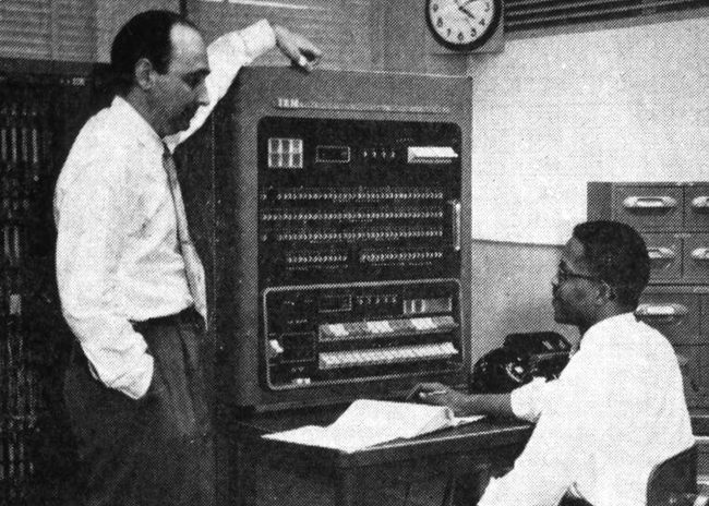
On the morning of 6 May 1955, in a former Census Bureau building on the south-eastern fringe of Washington, D.C., a thirty-five-year-old MIT-trained meteorologist named Frederick Gale Shuman stood next to an IBM 701 and watched the first operational numerical weather forecast in the United States come out of an oscilloscope-and-Williams-tube machine that had been built three years earlier in a former necktie factory at Poughkeepsie as the Defense Calculator. The seated operator at the console was a fellow Weather Bureau employee named Otha Fuller. The machine was rented from IBM at roughly two hundred thousand dollars a year – half the annual budget of the unit that had moved into the building eleven months earlier. The unit was called the Joint Numerical Weather Prediction Unit (JNWPU), formed by joint agreement of the U.S. Weather Bureau, the Air Force, and the Navy on 1 July 1954. Its first director was George P. Cressman, who had recruited Shuman as the unit’s first employee and chief modeller. The 701’s mean time between failures was about thirty minutes. The forecast that came out of it that morning – a 36-hour barotropic prediction of 500-hPa heights over the Northern Hemisphere – was not a particularly good forecast. The fact that the United States had one at all was a turning point.
The thirty-five-year-old at the 701 console that morning would, twenty-six years later, retire as the longest-serving director the unit’s institutional successor would ever have. In the months before he left he had personally authorised the operational deployment of a numerical method that would still be running on the National Weather Service’s computers nearly four decades after he walked out the door. This is the story of the seventeen years between those two events: April 1964 to January 1981, the directorship of Frederick Gale Shuman at the National Meteorological Center.
The thesis of the post is that an institutional director with a 1951 MIT doctorate, a Korean-era Air Force reserve commission, and a stubborn operational temperament built – in a Maryland office building two miles down the road from the original 1954 JNWPU site – the computing and modelling infrastructure that carried United States operational weather forecasting through three computer generations, four model lineages, and one architectural pivot from finite differences to spherical harmonics. The infrastructure outlived him by four decades. The Limited Area Fine Mesh model he commissioned in 1969-1970 was still running operationally in 1994. The Global Spectral Model he authorised five months before he retired ran continuously, in its descendant lineage, until 12 June 2019. The smoothing operator he wrote down in 1957 is still cited in atmospheric-modelling textbooks in 2026.
Where Post 39 left off
Our previous post on the spectral transform told the global story of how William Bourke’s Australian spectral primitive-equation model – the multi-level extension of the transform method that Bourke welded together in Melbourne in 1972 and 1974 – propagated outward to every major operational forecasting centre on Earth between 1980 and 1993. The post’s central operational landmark was the August 1980 debut of Joseph Sela’s R30L12 spectral model at the United States National Meteorological Center, the first operational deployment of the Bourke-Hoskins-Simmons formulation at any major weather centre. The spectral GFS lineage that began that month ran for thirty-eight years, eleven months, and three weeks before being retired on 12 June 2019 in favour of GFDL’s finite-volume cubed-sphere core.
What that post did not tell was the American institutional story of who decided to let it happen, and what the National Meteorological Center had been running before it. The answer is: a sixty-four-year-old man who had spent his entire career at Suitland, who had run his first operational model on the IBM 701 in 1955, who had been chief modeller of the JNWPU under Cressman from 1954, and who had been the Center’s own Director since April 1964. By the standards of operational atmospheric science he was an unusually long-tenured administrator. He had personally seen every model the Center had run from 1955 to 1981. He had personally written several of them. When Sela’s spectral model went operational in August 1980, he was the man who signed off on it. Five months later he retired.
This is the story of those five months, and of the seventeen years that led up to them.
A Hoosier at the IAS
Frederick Gale Shuman was born on 13 July 1919 in South Bend, Indiana, in the second year of the influenza pandemic. His high-school years were spent at South Bend Central, where in 1937 he won first place in the Indiana statewide comprehensive mathematics competition. He took his bachelor’s degree in mathematics at Ball State University in Muncie in 1941, working part-time as a junior weather observer at the Indianapolis Airport while still completing the degree. The Weather Bureau had a small operational presence at most major American airports by the late 1930s – a single observer reading the cloud height, the wind, the surface pressure, the precipitation, and dictating the observation to a teletype operator who sent it out on the airway weather-reporting circuit. Shuman, twenty-one years old in the summer of 1941, was one of those observers.1
The Second World War arrived in December and reorganised the Weather Bureau into an Army-Air-Corps-supporting branch of operational forecasting. Shuman, by then a Weather Bureau employee in good standing with a mathematics degree, was commissioned a second lieutenant and sent to MIT, which between 1941 and 1945 ran the Army Air Corps’s pipeline meteorology programme for officers who would forecast the European, African, and Pacific theatres. He took an M.S. in Meteorology at MIT in 1942 and was deployed as a weather officer to the North African and Italian theatres for the remainder of the war. He was discharged from active duty in 1945 and held the rank of major in the Air Force Reserve when he was finally fully discharged in 1956.
After the war he returned to the Weather Bureau as an airways forecaster at the Wayne County Airport in Detroit, then transferred to the Bureau’s Washington research division to work on the early severe-storm and tornado-forecasting problems that were just beginning to be amenable to systematic study. By 1951 he was back at MIT, finishing the doctoral work he had begun before the war. His dissertation, defended in 1951, is the first doctoral thesis on numerical weather prediction at MIT, on the evidence of the Wikipedia biographical article. The thesis advisor is not in any of the open biographical sources I have been able to consult; given the period and the topic, the standard candidates would be Sverre Petterssen, Bernhard Haurwitz, or one of the senior MIT meteorology faculty of the late 1940s. The degree was a Doctor of Science (Sc.D.), MIT’s specific term of art for what most American universities call a Ph.D.2
The Sc.D. degree took him directly to the Institute for Advanced Study at Princeton, where between 1952 and 1954 he worked on numerical weather prediction in the immediate aftermath of John von Neumann and Jule Charney’s first integrations of the atmosphere on the IAS machine. The IAS computer – the electronic stored-program machine that John von Neumann had championed against the resistance of the Princeton mathematics department, with Julian Bigelow as chief engineer and Herman Goldstine as scientific director – had run the famous Thanksgiving 1950 baroclinic-model forecast that demonstrated, for the first time, that the equations of atmospheric motion could be solved fast enough to overtake the weather. By the time Shuman arrived in Princeton, the IAS machine had been running for two years; von Neumann was alive (he would die of cancer in 1957); Charney was the senior atmospheric scientist on the project. The Mariners Weather Log obituary records that Shuman attended lectures by J. Robert Oppenheimer – IAS Director from 1947 to 1966 – and by Albert Einstein, who was a Professor of Theoretical Physics at IAS until his death in April 1955. The lectures by Oppenheimer would have been in the years before his June 1954 security-clearance revocation. The lectures by Einstein are the more remarkable detail: Shuman was the youngest of perhaps a half-dozen Weather Bureau staff who heard Einstein, in person, in the last two years of his life.3
What Shuman took from the IAS years was the working knowledge of a 1952-era stored-program computer (in the obituary it is loosely called the JOHNNIAC, but JOHNNIAC was the RAND copy of the IAS machine; what Shuman actually ran on was the IAS machine itself, or one of its sister implementations), an apprenticeship in the von Neumann-Charney programme of numerical-weather-prediction theory, and a set of personal contacts inside the Princeton group that he would draw on for the rest of his career. He was, by mid-1954, a thirty-four-year-old MIT-trained meteorologist with operational Weather Bureau experience, an MIT doctorate on a numerical-weather-prediction topic, two years of stored-program-computer experience at the IAS, and an Army Air Corps reserve commission with formal Pentagon ties. When George Cressman – then a senior Weather Bureau staff scientist who had been negotiating the inter-service agreement that would create the JNWPU – went looking for a chief modeller for the new operational unit at Suitland, Shuman was the natural choice. The Find a Grave memorial calls him the unit’s first employee.4
The 1955 forecast and the three years of disappointment
The Joint Numerical Weather Prediction Unit was formally established by joint agreement of the Weather Bureau, the Air Force, and the Navy on 1 July 1954. Cressman was its first Director. Shuman was its chief modeller. The unit occupied space in Federal Office Building 4 (FOB-4) at the Suitland Federal Center, Suitland, Maryland – a 1942 Census Bureau building about ten kilometres south-east of the Capitol. The IBM 701 was installed in March 1955. The first experimental forecasts began in April. The first operational issued forecast went out on 6 May 1955.5
The forecast was not good. Cressman, writing forty-one years later for the AMS Historical Essays volume, was honest about how thoroughly the unit had under-estimated the difficulty of operational numerical weather prediction:
“[The early model’s results] were not nearly as good as the earlier tests had indicated. It had not occurred to us that we could have success with [the] very difficult baroclinic events [studied during testing] and then have severe problems with many routine, day-by-day weather situations.”
Shuman in 1989, in his own retrospective for Weather and Forecasting, gave the same verdict more compactly:
“Within three years three agencies of the United States Government jointly created a numerical weather prediction service, but it was quickly discovered that current models had very serious defects. After considerable research, the first operationally effective model was achieved in 1958.”6
What happened between 1955 and 1958 is the un-romantic version of the operational numerical weather prediction story. The unit retreated from the three-level baroclinic model that had been its showpiece to a two-layer baroclinic model in 1956, then back to a simple barotropic model based on the original ENIAC code – the same code that Jule Charney’s group had run at Aberdeen Proving Ground in March 1950, restricted to one vertical level and one prognostic equation. By 1958 that simpler model had been refined enough to be operationally useful. The IBM 704 (1957), the IBM 7090 (1960), the IBM 7094 (1963), and the CDC 6600 (1966) replaced one another at FOB-4 in turn, each more capable than the last. The unit’s institutional structure was reorganised on 1 January 1958: the JNWPU was merged with the National Weather Analysis Center (NAWAC) to form the National Meteorological Center (NMC). Shuman became Chief of the new Center’s Development Division. Cressman remained Director.
The three-level baroclinic model was reintroduced operationally in 1962. As Paul Edwards put it in his 2010 A Vast Machine, “this model initially offered only slight improvements over the barotropic forecast”; the operational community was now beginning to grasp that the gap between theoretical elegance and operational usefulness was wider than the von Neumann-Charney generation had imagined.7 Shuman’s first major individual contribution was a methodological one published in this same period, and – in a pattern that recurs throughout his career – the contribution was directed at the un-romantic problem of making the operational machinery actually work.
The Suitland filter
The two papers Shuman published in the November 1957 Monthly Weather Review were titled with characteristic Weather-Bureau understatement: “Numerical Methods in Weather Prediction: I. The Balance Equation” and “Numerical Methods in Weather Prediction: II. Smoothing and Filtering.”8 The first paper dealt with the elliptic-equation problem of computing balanced wind fields from a given mass field on the operational analysis grid – a standard initialisation step in primitive-equation modelling. The second paper, which has come to be known as the Shuman filter, is the one that has outlived its author.
The Shuman filter is, in plain language, a numerical-recipe trick for smoothing operational gridded fields without distorting the patterns the forecaster cares about. The technical statement is that it is a weighted-average operator – a five-point or three-point running mean – with coefficients chosen so that the operator’s frequency response is approximately zero at the smallest wavelength the grid can represent (the two-grid-point wave, in finite-difference jargon) and approximately one for the meteorologically significant scales (the eight-grid-point wave and longer). The operator suppresses the saw-tooth noise that finite-difference primitive-equation integrations accumulate near the grid’s truncation cutoff, without touching the synoptic patterns the analysis is supposed to show.9
A musical analogy may help. A poorly-recorded vinyl record has surface hiss – high-frequency noise that overlays the music. A graphic equaliser with a high-cut filter rolls off the top end of the spectrum without touching the midrange where the music lives. The Shuman filter is the operational-meteorology equivalent: it rolls off the noise at the smallest scales that the grid resolves, where the finite-difference scheme is most likely to be lying, and leaves the larger scales – the ones the forecaster is reading off the chart – essentially unchanged. The mathematical novelty is the design philosophy: specify the desired frequency response, then derive the finite-difference weights that approximate it. This was the inverse of the more usual approach of writing down an averaging stencil and then computing what its response happened to be. The 1957 paper gives the explicit table of weights and the demonstration of the response curve.
The filter became standard practice in operational numerical weather prediction within a decade. It was cited and used not only at NMC but at every major operational centre that ran finite-difference primitive-equation models in the 1960s and 1970s. The standard atmospheric-modelling textbook of the operational community – Fedor Mesinger and Akio Arakawa’s Numerical Methods Used in Atmospheric Models (GARP Publications Series No. 17, 1976) – includes the Shuman 1957 paper among its canonical references. Dale Durran’s Numerical Methods for Fluid Dynamics (Springer 2010), forty-three years after the original publication, still cites it as the foundational reference for finite-difference smoothing operators in atmospheric science. The filter even propagated outside meteorology: two papers in the Journal of Engineering Mathematics in 1980-1981 – “The Shuman filtering operator and the numerical computation of shock waves” and “Switched numerical Shuman filters for shock calculations” – adopted the construction for computational-fluid-dynamics shock calculations.10
In 2026 the Shuman filter is no longer in the inner loop of the major operational global models. The spectral GFS used spectral truncation as its principal noise control; the present-day FV3 GFS, the ECMWF IFS, the UK Met Office’s Unified Model, ICON, and the JMA GSM all use higher-order numerical diffusion schemes that have superseded the 1957 filter for production use. But the filter is still a teaching reference, still cited in the introductory textbooks, still implemented in the legacy archive-processing code that the Climate Forecast System Reanalysis and similar long-record products run on. Sixty-nine years after publication, it is, by most accountings, the longest-lived single numerical-recipe contribution any individual American operational meteorologist has put into the literature. Shuman was thirty-eight when he wrote it.
April 1964
George Cressman was named Director of the Weather Bureau in 1965 after the federal reorganisation that created the Environmental Science Services Administration (ESSA, the immediate ancestor of NOAA). His move to the Weather Bureau headquarters left the NMC directorship vacant a year earlier; Shuman, by then Chief of the Development Division and the institutional memory of the Center’s first decade, was promoted to Director of the National Meteorological Center in April 1964. He was forty-four years old. He would hold the post for seventeen years.11
A small factual note on the date. Several otherwise authoritative sources – including the WPC’s own 2025 institutional history PDF and the Mariners Weather Log December 2007 profile – date the promotion to April 1964, and Wikipedia, the Washington Post obituary, and the Find a Grave memorial agree. Some secondary accounts have the date as 1965, confusing the NMC directorship with the simultaneous Weather Bureau reorganisation. The right date is April 1964.
The Center that Shuman inherited was not the Center it would become under his directorship. In April 1964 NMC occupied space at FOB-4 Suitland alongside its sister units (NESS, the National Environmental Satellite Service; the Weather Bureau Forecast Office for Washington D.C.; the auxiliary climate and analysis groups). Its principal computer was the IBM 7094, then four years old, soon to be supplanted by the CDC 6600 that was ordered in 1964 and installed in 1965-1966. The operational forecast suite was three-level baroclinic on a 381-kilometre-resolution Northern-Hemisphere grid. The first global primitive-equation model had not yet been built. The first regional fine-mesh model had not yet been built. The first operational data-assimilation cycle had not yet been built. By the time Shuman retired, in January 1981, all three would exist as operational systems, two of them named after him.
The first thing he did, in 1966, was build a model.
The six-layer PE
The Shuman-Hovermale six-layer primitive equation model went operational on the CDC 6600 in June 1966. It was the first operational primitive-equation model anywhere in the world. The 1968 paper that documents it, in Journal of Applied Meteorology 7(4): 525-547, is the canonical citation:
“In its first fourteen months of operational use, it has resulted in highly significant improvements in the Center’s products.”12
The co-author was John B. Hovermale (1939-1994), a Penn State-trained dynamicist who would build NMC’s first operational hurricane model nine years later. The model was a clean break from the quasi-geostrophic and quasi-vorticity approximations that had constrained every operational NWP system since the 1950 ENIAC integration. The full hydrostatic primitive equations – conservation of momentum, conservation of mass, conservation of energy, the hydrostatic balance, and the moisture equation – were integrated directly. The vertical structure was six sigma layers, with the boundary layer represented as the lowest two. The horizontal grid was an octagonal polar-stereographic mesh covering most of the Northern Hemisphere from 10 degrees north to near the pole, with grid points roughly 381 kilometres apart at 60 degrees north. The hemispheric integration ran twice daily, at 00 and 12 UTC, on the CDC 6600.
West Germany’s Deutscher Wetterdienst was working on a comparable primitive-equation system in parallel; the Hamburg group went operational a few months later in 1966. The two systems were the world’s first two operational primitive-equation models, by an institutional gap of months. Edwards (2010, p. 129) reproduces the model’s grid diagram with the source attribution to the 1968 paper; the figure has been propagating through atmospheric-modelling textbooks for fifty-eight years as the canonical example of an octagonal polar-stereographic operational grid.7
The Shuman-Hovermale model is the foundation on which the post’s central decade-and-a-half rests. It was, until August 1980, the principal hemispheric forecast product of the United States National Weather Service. It carried NMC through the CDC 6600 (1966-1971), the IBM 360/195 era (from approximately 1971 onward; see below), and the start of the spectral transition. Successively upgraded – to higher vertical resolution, to semi-implicit time integration, to a finer horizontal grid – it was the senior operational model on the FOB-4 production floor for fourteen years. Shuman’s name on the paper was, in retrospect, the most consequential of the four operational models that ran during his directorship. It is also why the 1980 Charney Award citation – which we will come to in section eleven – explicitly mentions “primitive equations models” in the plural.
What the production floor actually had
This section is the structural backbone of the post, and it requires care, because the documentary record on what the National Meteorological Center actually owned and ran during the 1970s is in places mutually inconsistent. The honest summary is that NMC was running, throughout the second half of the decade, a homogeneous-architecture machine room of IBM System/360 Model 195 mainframes – with the exact count somewhere between one and three depending on which institutional source one trusts – inside FOB-4 at the Suitland Federal Center.
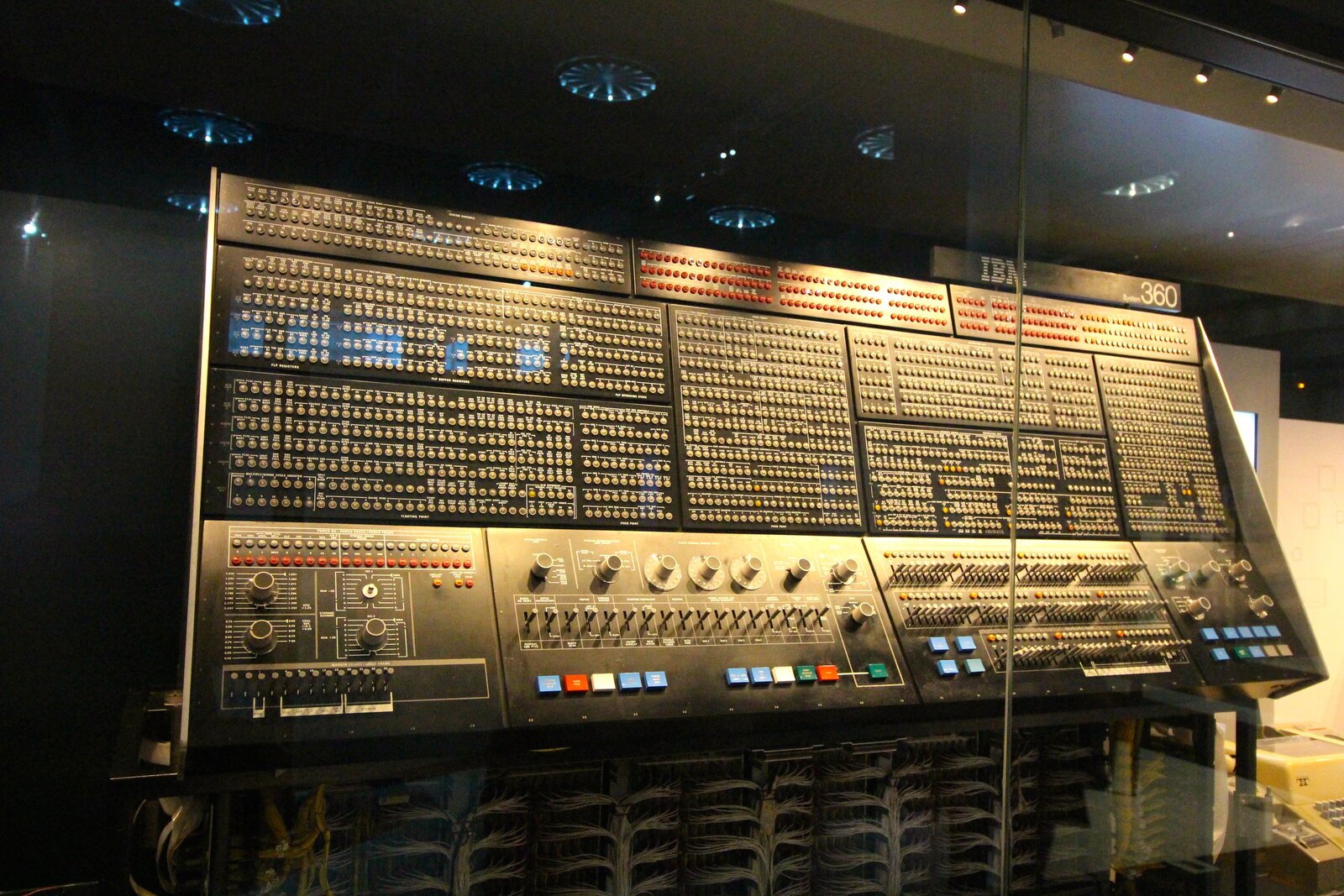
The 360/195 was IBM’s last entry in the supercomputer class until the 3090 series of the mid-1980s. It was announced on 20 August 1969 and withdrawn from marketing on 9 February 1977 – a production window of seven and a half years. Approximately twenty machines were built across the run. The 195 was, in microarchitectural lineage, a direct descendant of the System/360 Model 91 we covered in Post 31: it inherited the Tomasulo-algorithm floating-point unit with its reservation stations and common data bus, paired with a more conventional cache hierarchy and a 54-nanosecond CPU cycle. Peak floating-point throughput was about six megaflops per machine. The list price was between seven and twelve million 1969 dollars; monthly rental ran from 165 000 to 275 000 dollars depending on configuration. The 1971 figure of “first IBM 360/195 at NMC” from the AMS 2019 retrospective by Yang and Tallapragada places it within the production window; the WPC’s own institutional history dates “the high resolution PE model on an IBM 360/195” to 1978, which probably refers to the upgrade of the model rather than the original installation of the hardware.13
The documentary record on the number of 195s at NMC is more contested. The blog series itself, in Post 31, cites “three Model 195s, the first installed in March 1974 and the third in November 1975” – a count consistent with the Yang and Tallapragada 2019 retrospective, which lists “1972: 3 IBM 360-195s” on its computer-history slide at eighteen megaflops aggregate. The September 2025 WPC institutional history PDF, however, refers to “the IBM/195” in the singular; the 1986 NMC Product Suite document (Western Region Technical Attachment 86-05) likewise treats the machine as a single article; the 1984 conference paper by Dennis Deaven describing the Cyber 205 conversion uses the singular “the IBM/195” throughout. The most defensible single sentence is that the documentary record on the number of 360/195s at NMC is contested: later retrospectives say three machines, while contemporaneous documentation refers to them in the singular – most likely one production unit with development or backup machines bringing the count to two or three at peak. The fact that NMC was, in the second half of the 1970s, running a homogeneous IBM 360-architecture machine room of at least one and possibly three Model 195s as its operational backbone is not in dispute.
Where physically. FOB-4 (Federal Office Building 4), Suitland Federal Center, Suitland, Maryland. The building had been part of the Census Bureau complex since 1942. The JNWPU had moved in during the spring of 1955; NMC had been there since the January 1958 reorganisation. The 360/195s lived in the FOB-4 machine room. They would continue to live there until 1999, when an IBM SP cluster was installed at a new NCEP machine site in Bowie, Maryland.
Where the people were. This is the part of the institutional story that is easiest to miss. The World Weather Building at 5200 Auth Road, Camp Springs, Maryland – about two miles south-east of the FOB-4 machine room – was dedicated on 22 October 1974, four months into Shuman’s eleventh year as Director. NMC’s forecasters, analysts, and senior scientific staff moved into the new building on Wednesday, 19 February 1975, the day after Presidents Day. The bulk relocation is recorded in the testimony of employee Bill McReynolds in the NWS Heritage institutional memoir. The computers did not move with them. The 360/195s were too heavy, too power-hungry, and too tightly integrated with FOB-4’s chilled-water plant; the institutional decision was that the people would relocate and the model output would be transmitted electronically two miles down the road to the new building.14
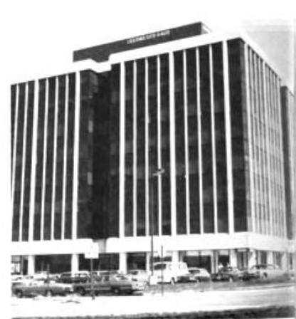
That distinction – the people at Camp Springs, the computers at Suitland – matters because it is the institutional fact behind the loose tradition in the secondary literature of calling NMC “the Suitland operation” through the late 1970s. Strictly, from February 1975, “Suitland” was the machine room; the forecasters’ offices were two miles away. The forecasters’ building was shared with the National Environmental Satellite Service, with the Washington Weather Service Forecast Office (Eugene Hoover and Jerrold La Rue ran the daily operational shift in 1974), and with the auxiliary climate and analysis units. The mainframes’ building remained the FOB-4 Census-Bureau-era structure, with the chilled-water plant and the raised-floor machine hall that had housed the IBM 701 in 1955.
Four times daily
By the mid-1970s NMC was running its operational analysis-and-forecast cycle four times a day, at the standard synoptic hours 00, 06, 12, and 18 UTC. The cycle was the institutional spine of every product the Center produced. Each six-hour cycle consisted of three stages. The first stage was the objective analysis, which combined the previous cycle’s six-hour forecast (the first guess) with all the observations available within the cycle window (radiosondes, surface stations, ship reports, aircraft reports, and, after the late 1970s, satellite temperature retrievals). The second stage was the initialisation, which adjusted the analysis to satisfy the model’s balance constraints. The third stage was the forecast integration, which produced the next cycle’s first guess and, for the principal cycles at 00 and 12 UTC, the full operational forecast suite out to 48 or 72 hours.
The objective-analysis methodology evolved across Shuman’s directorship in three steps. The earliest method was the Cressman successive correction scheme, the 1959 paper by NMC’s first Director that introduced an iterative algorithm: apply a correction at each grid point that is a weighted average of nearby observation increments, with the correction radius shrinking on each successive pass. The Cressman scheme was simple, fast, and conservative; it remained NMC’s primary analysis method into the early 1970s. The second method was Hough analysis, introduced in 1971 by NMC’s Thomas Flattery. Hough functions are the solutions to Laplace’s tidal equations on a rotating sphere – a special set of orthogonal basis functions adapted to atmospheric motions, used here as the interpolating basis. The advantage was that the Hough basis treated mass and motion fields self-consistently, removing the spurious imbalances that the Cressman scheme could introduce. Hough analysis was operational for some products from 1971 through the early 1980s.15
The third and decisive method was optimum interpolation, the technique that came to NMC at the end of the 1970s. The seminal NMC paper is McPherson, Bergman, Kistler, Rasch, and Gordon, “The NMC operational global data assimilation scheme,” Monthly Weather Review 1979. The first author is Ronald D. McPherson, NMC’s lead data-assimilation scientist throughout the late 1970s and, fifteen years later, the Center’s Director (1990-1998). Optimum interpolation is a statistical-estimation method: at each analysis grid point, the analysed value is a linear combination of the first-guess value and nearby observation increments, with the weights chosen to minimise the expected analysis error variance given assumed covariance structures for the background and observation errors. It is the operational forerunner of the variational and ensemble methods that came to dominate operational data assimilation from the mid-1990s onward.16
The McPherson et al. paper appeared in Monthly Weather Review in 1979. NMC’s full Global Optimum Interpolation (GOI) for the operational global system entered operations through 1979 and 1980. The pacing event was FGGE.
FGGE 1979
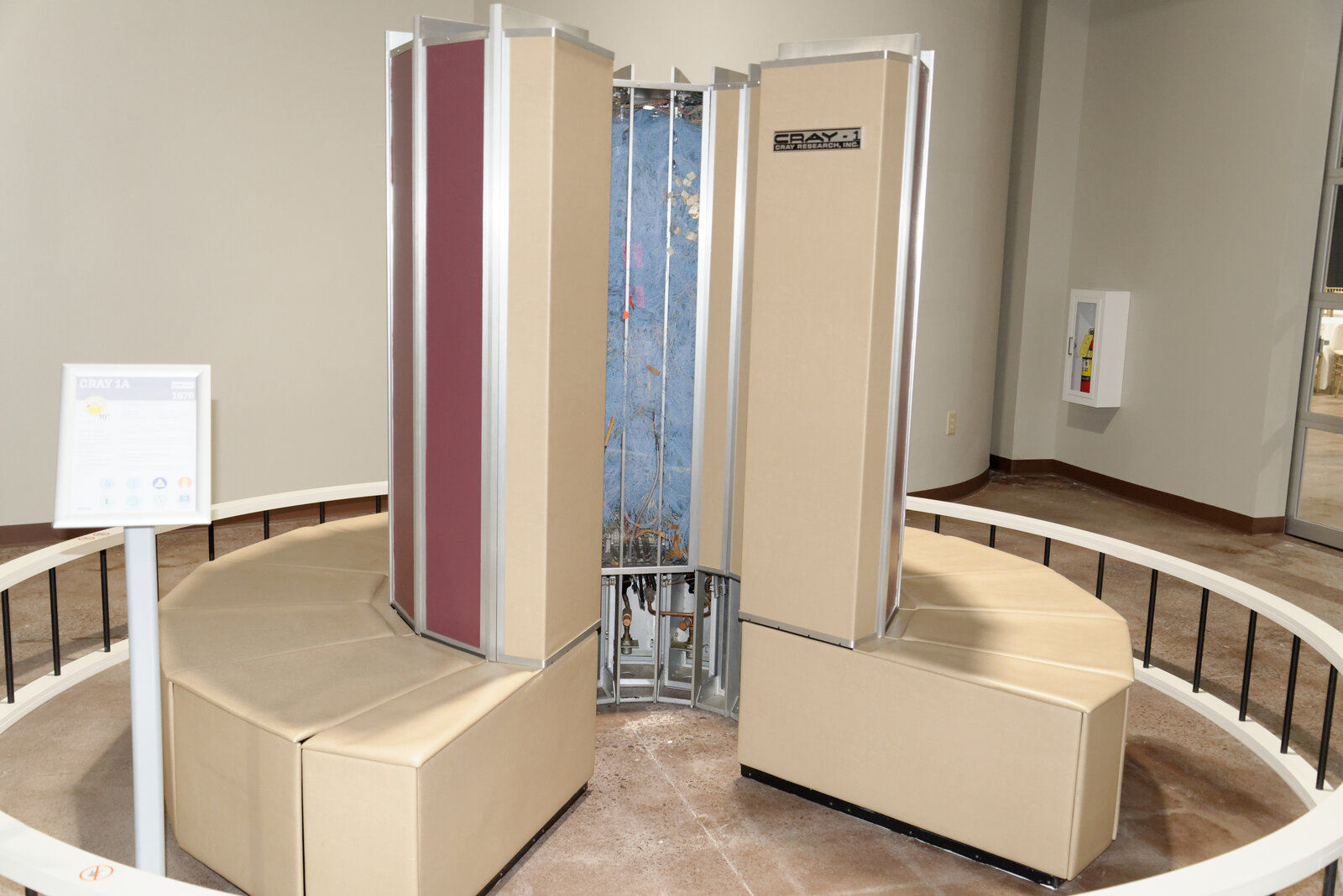
The First GARP Global Experiment – FGGE, or sometimes “the Global Weather Experiment” in the open American literature – was the largest international observational programme of the 1970s. The two Special Observing Periods, SOP-1 from January to March 1979 and SOP-2 from May to June 1979, deployed dropwindsondes, drifting buoys, geostationary satellite imagery, additional radiosondes, and – the genuinely new thing – the first concentrated effort to assimilate satellite temperature retrievals from the TOVS/HIRS instrument suite into operational global analyses. NMC was the United States analysis centre for the experiment; ECMWF, then less than four years old in its Reading offices and running the Cray-1A serial number nine we covered in Post 34, was its European counterpart. The two centres’ parallel operational analyses for the FGGE periods are still cited as foundational reanalysis datasets in atmospheric science.
The operational pacing of NMC’s GOI implementation was driven by FGGE. The McPherson et al. paper was written in 1978 and published in 1979 specifically because the operational system had to be in place to handle the unprecedented data volume of SOP-1 in January. The decision was Shuman’s; the technical execution was McPherson’s. The FGGE-era data flow at NMC ran on the Suitland 360/195 production floor, with the model output transmitted to Camp Springs for the operational shift. The institutional memory of FGGE inside NMC is the more important fact than any specific product: the experiment proved, to the operational community’s satisfaction, that four-dimensional global data assimilation could be done at production scale on the hardware then available.
The LFM
The Limited Area Fine Mesh model is the operational artifact that most clearly bears the Shuman directorship’s institutional fingerprint, partly because of its 1971 operational debut, partly because of its survival until 1994 – thirteen years after Shuman retired and four years after every senior NMC scientist who had worked on it had left the Center. The LFM was a regional primitive-equation model on a polar-stereographic grid covering North America, designed to give forecasters short-range numerical guidance available two hours after synoptic time – much earlier than the Center’s primary operational model could deliver. The acronym was originally L for Local; it was redefined as L for Limited-area during development. The model survives in the institutional memory under the second meaning.17
The LFM’s mathematical lineage went back to John G. Howcroft’s 1971 NMC Office Note 50, “Local Forecast Model: Present status and preliminary verification” (23 pp.). Howcroft’s 1966 conceptual notes are sometimes cited as the starting point but Office Note 50 is the operational specification document. The model was deliberately a fine-mesh sibling of NMC’s then-operational Shuman-Hovermale hemispheric model, at half the parent model’s grid length. Rocky Hirano’s April 1994 NMC Office Note 404 – the LFM’s institutional epitaph, published in the same month the model was retired from operations – is explicit on the design intention:
“This model was to be constructed in a similar manner as NMC’s operational model, the Six-Layer Primitive Equation (6LPE); it was to run about two hours after synoptic time, over a limited area, and with a grid length one-half of the 6LPE, at 190.5 km.”17
The LFM began operational 24-hour forecasts on 29 September 1971, on what was by then the CDC 6600 production hardware (the 6600 would not be retired until later in the 1970s, running in parallel with the incoming 360/195s during the transition). The grid was 53 by 57 points – 3 021 points in total – on a polar-stereographic projection true at 60 degrees North, with 190.5-kilometre spacing at the projection’s tangent latitude. The vertical was six sigma layers: a boundary layer, three tropospheric layers, and two stratospheric layers with an isentropic cap. Two early adjustments are in the institutional record. The first, on 7 February 1973, removed twelve grid rows over the polar region, reducing the forecast grid to 53 by 45 (2 385 points) for runtime efficiency. The second, in the first quarter of 1975, extended the forecast cycle from 24 hours to 36; in December 1975 it was extended further to 48.
A small dating note: the brief flagged a discrepancy between the LFM/Sela research file (29 September 1971) and the broader Shuman biographical research file (31 October 1971) for the operational debut. The Hirano 1994 Office Note 404, which is the LFM’s own institutional retrospective written by its long-serving developer, is unambiguous on 29 September. The 31 October date in some secondary sources is plausibly the day operational forecasts began for the NCAR-archived LFM dataset (the NCAR Data Support Section’s temporal-coverage records start on 31 October 1971). The two dates are compatible: 29 September was when the model began operational issue at NMC; 31 October was when NCAR began routinely receiving and archiving the operational output. The text above gives the NMC operational debut date, the one that matters for the Shuman directorship’s institutional record.17
The model went through two further major upgrades during Shuman’s tenure. The first was the LFM-II implementation on 31 August 1977, which halved the horizontal mesh from 190.5 kilometres to 127 kilometres – three grid points where the original LFM had two. The original 190.5-kilometre grid was retained for analysis and display; the forecast and post-processing ran on the 127-kilometre mesh. The second upgrade, on 1 March 1979, introduced the seven-layer LFM (boundary layer + three tropospheric + three stratospheric), documented by J. E. Newell in the NMC Atmospheric Modeling Branch bulletin of 22 January 1979.18 The final major Shuman-era modification was the LFM-II “in-core” version that became operational on 10 June 1981 – five months after Shuman had retired but on the production track that had been set up under his directorship. The in-core LFM reverted to 190.5-kilometre resolution but introduced fourth-order finite-difference numerics; Hirano notes explicitly that “forecast quality remains essentially unchanged after 1981 when the last major modification was implemented.”
The LFM was first guidance, not best guidance. It ran with a data cutoff one and a half hours after synoptic time – earlier than any other operational model at NMC – so the forecasters had something on their desks by mid-morning for the 00 UTC cycle and by mid-evening for the 12 UTC cycle. Its forecast quality was characterised by Hirano as “essentially unchanged” from 1981 onward, neither improving nor deteriorating. By the late 1980s the LFM was no longer the most skillful regional model at NMC – the Nested Grid Model (NGM) built by Norman Phillips had been operational since 1985 at higher resolution, and the Eta model of Fedor Mesinger and Zaviša Janjić would become operational in June 1993 and surpass it on most skill metrics. But the LFM ran. It came out first. The forecasters had been using it for twenty years.
Long operational tails
The LFM was retired – removed from operations – in April 1994, per Hirano’s Office Note 404 dated that month:
“[The LFM] contributed significantly to the quality of NMC forecast products principally during the decade after implementation in 1975. Thereafter, it served as the first guidance available to forecasters after synoptic time until it was removed from operations this year.”17
The “this year” in Hirano’s text refers to 1994, the year the office note was published. The exact month within 1994 is not in the text; the office note’s April 1994 dating and its use of the past tense to describe the LFM suggests retirement in the first quarter of 1994. The Eta model had become operational on the principal “Early” run in June 1993; the LFM survived another year past that as a parallel-run backup, then was retired.
The total operational lifespan of the LFM is therefore 29 September 1971 to early 1994 – approximately twenty-two and a half years. The model was on operational duty at the National Meteorological Center for the entire second half of Shuman’s directorship (October 1971 to January 1981) and for thirteen additional years after Shuman’s retirement. It survived the Cyber 205 procurement of 1981-1983 (port to the new hardware by Dennis Deaven, operational on the Cyber 205 by 30 August 1983); it survived the introduction of the Nested Grid Model in 1985; it survived Phillips’s 1988 retirement, McPherson’s 1990 promotion to the Center’s directorship, and the early Eta development. Hirano’s notes preserve the institutional reason for the longevity in two specific findings.17
The first finding is the earliest-product advantage. The LFM was the first regional forecast available each day. Even when the NGM (1985) and the Eta (1993) became operational, the LFM was still the first product into the forecasters’ hands. Operational forecasting culture cared about the morning briefing – the time-pressured composition of the day’s predictions for distribution to airline dispatchers, military weather offices, and the public-affairs branch of the National Weather Service. The first regional forecast to land on the operational chart desk shaped the framing of the day’s discussion, whether or not it was the most accurate.
The second finding is the known-quantity advantage. Hirano’s S1-score time series for the LFM is, from 1981 onward, almost flat. The model neither improved nor deteriorated. Forecasters knew its biases: it under-predicted Great Lakes lake-effect snow, it over-predicted Appalachian orographic precipitation, it had specific failure modes in coastal cyclogenesis off the Atlantic seaboard. They corrected for those biases on the chart desk. When a newer, more accurate model arrived – the NGM, the Eta – the forecasters had to learn its biases, which were different. The LFM had the consistency of an old instrument: imperfect, but predictable in its imperfections.
The pattern – long operational tails on legacy models, defended by forecaster preference and known-bias correction – is one we encountered in the previous post on spectral methods. The R30L12 spectral GFS of August 1980 took thirty-eight years and eleven months to be retired, fifteen of those years after the architectural community had recognised that the spectral method was no longer the obvious choice for the dominant operational architecture. The LFM took twenty-three years to retire, nine of those years after the NGM had surpassed it on most skill metrics. Code that took fifteen years to write took two decades to retire. The LFM’s history is the regional-scale instance of the same institutional pattern.
The last decision
Shuman’s last major architectural decision was the one that retroactively justifies the post’s framing of his directorship. It was the authorisation to deploy Joseph Sela’s global spectral model in operations.
Joseph G. Sela – born in Israel, educated in Israel and then in the United States in the 1960s, attached to NMC’s Development Division from 1975 onward, husband of Malca Sela and father of Rafael and Amir – is one of the more important institutional figures in the post-war American operational weather-prediction community.19 He joined NMC in 1975, when Shuman was eleven years into his directorship, and was given the assignment of porting the new spectral primitive-equation methodology that William Bourke had published in 1974 and Brian Hoskins and Andrew Simmons had published in 1975 to the NMC operational suite. His office was at FOB-4. His machines were the 360/195s. His physics package was lifted essentially intact from Shuman and Hovermale 1968 – the same primitive-equation parameterisations that the operational hemispheric model already used. His sigma vertical coordinate was Phillips 1957. His finite-difference vertical scheme was the Arakawa-Mintz quadratic-conserving formulation of 1974. The only thing genuinely new about Sela’s model, relative to what NMC was already running, was the horizontal dynamics: spectral, not finite-difference; spherical harmonics, not octagonal polar-stereographic grids.
I want to slow down at this point and be precise about what Sela’s model actually was, because earlier briefings on the topic in this series contained a small but consequential error of memory.
The model’s resolution is R30L12: rhomboidal truncation at 30 waves, L12 = 12 sigma levels. The “R” matters. Triangular truncation – the convention that becomes universal in the global spectral literature by the late 1980s – did not arrive at NMC until August 1987, when William Bonner’s directorship pushed the resolution to T80L18 (triangular truncation at 80 waves, 18 sigma levels) on the Cyber 205. The August 1980 model was rhomboidal. The blog series has sometimes written “T30L12” by reflex from later spectral practice; the correct label for Sela’s operational debut is R30L12. (Equivalent grid spacing at 60 degrees North: approximately 375 kilometres – comparable to the Shuman-Hovermale 381-kilometre grid that the spectral model was about to replace.)
The model’s name is Sela’s. There is no “Joel Tenenbaum” at NMC; an earlier memory-note conflation between Sela and a real Purchase College meteorologist of similar surname has been corrected in this series’s research files. Joseph G. Sela was the sole institutional lead of the NMC spectral development from 1975 to operations, with contributions from the NMC Atmospheric Modeling Branch on the physics side. His own canonical journal-paper documentation is Sela 1980 in Monthly Weather Review 108: 1279-1292 (“Spectral Modeling at the National Meteorological Center”); the corresponding technical report is NOAA Technical Report NWS 30, The NMC Spectral Model, 38 pages, published in May 1982 – eighteen months after the operational debut.20
The operational rollout was two-staged. On 27 May 1980 the spectral R30L12 model was implemented in the Global Data Assimilation System (GDAS), running in parallel with the operational gridpoint primitive-equation analysis-forecast cycle. The implementation included the non-linear normal-mode initialisation of Machenhauer 1977 and Ballish 1981, which adjusts the analysis to the model’s gravity-wave balance in spectral space rather than on a grid. In August 1980 – the exact day-of-month is not in the open documentary record – the spectral model entered operational production in the AVN (Aviation, 144 hours) and MRF (Medium Range Forecast, 240 hours) products. The first August 1980 forecast was generated on the FOB-4 360/195s.21
The operational forecast configuration was unusual by modern standards because the 360/195 hardware did not have the throughput to run the spectral model at full resolution out to 240 hours within the operational window. Sela’s solution was to reduce the resolution as the forecast extended:
- At 48 hours: horizontal resolution reduced from R30 to R24 waves.
- At 144 hours: vertical resolution reduced from L12 to L6.
- At 192 hours (8 days): the domain reduced from global to Northern Hemisphere only.
The full-resolution R30L12 was therefore reserved for the principal short-range forecast, with progressively coarser resolutions covering the medium-range and extended-range products. The trade-off was Sela’s own engineering judgement: spectral resolution where it mattered most, scalar computational economy where the forecast skill was already declining with forecast hour.
What is worth emphasising for the institutional argument of this post is that the operational debut of the spectral model in August 1980 happened five months before Shuman’s retirement in January 1981. Shuman explicitly authorised the deployment. The decision was contested at the procurement and technical levels: spectral models were substantially less computationally efficient than finite-difference primitive-equation models on scalar-architecture machines like the 360/195, and a defensible operational choice would have been to wait for the new Cyber 205 (the procurement of which was already in progress at NOAA) before deploying the new architecture. Shuman’s authorisation to deploy the spectral model on the existing 360/195 hardware was, in this sense, a bet that the upcoming Cyber 205 procurement would deliver vectorised throughput that the new method needed to make its eventual operational case. The bet paid off three years later.
October 1983, August 1987
The post’s title is Seventeen Years at Suitland, and by the standards of strict institutional chronology the story ends in January 1981 when William D. Bonner, of UCLA’s Department of Meteorology and the author of the 1968 MWR paper on the climatology of the Great Plains low-level jet, takes over as the Center’s third Director. But the relevant arc of Shuman’s last operational decision – the spectral procurement – carries forward another six and a half years before it reaches its first stable equilibrium, and the section title acknowledges that the seven years immediately after January 1981 are the years during which Shuman’s last decision became the operational architecture of the Center.22
1981 is the architectural pivot year. NMC took delivery of its first CDC Cyber 205 – the vector supercomputer that we covered briefly in the spectral post – through the year. The exact installation date is contested in the secondary literature: the Yang and Tallapragada 2019 retrospective slide lists “1981: CDC Cyber 205, 400 megaflops” as the year-of-installation; the 1984 Deaven conference paper “Operational Numerical Weather Prediction on the Cyber 205 at the National Meteorological Center” implies later acceptance testing; the WPC’s September 2025 institutional history PDF omits the Cyber 205 entirely from its institutional summary, listing only the IBM 360/195 followed by the Cray Y-MP8 of the late 1980s. The Deaven 1984 paper is the contemporaneous primary evidence and is unambiguous on the Cyber 205’s operational presence at NMC by 1983; the WPC summary’s omission probably reflects the Cyber 205’s role as an R&D and second-shift machine rather than the primary operational production stream.23
The first major operational milestone on the Cyber 205 was the LFM port – Dennis Deaven’s hand-vectorised conversion of the LFM-II inner loops to the Cyber’s 64-element vector pipelines, completed by 30 August 1983. The Cyber 205 LFM ran in 75 seconds for a 48-hour forecast, compared with 1 125 seconds on the IBM 360/195: a factor-of-fifteen speedup. The Deaven paper documents the conversion effort as “about a month and a half” of work by a single meteorologist-programmer – which is, by 1984 supercomputing standards, very fast, and reflects the structural simplicity of the LFM’s primitive-equation inner loop relative to more complex modern models.23
The second major Cyber 205 milestone is the one Shuman’s spectral procurement decision had been targeting. In October 1983, three years after the R30L12 operational debut, NMC upgraded the spectral resolution to R40L12 on the Cyber 205. The upgrade was made operationally affordable by the introduction of the highly-optimised Fast Fourier Transforms of Clive Temperton at the UK Met Office, which had been published in Journal of Computational Physics in 1983 and which became the standard FFT library for vectorised spectral models for the rest of the decade. R40 had about 78 per cent more horizontal grid points than R30 at the same vertical resolution; the operational improvement in 1983 was substantial. The R40L12 configuration ran on NMC’s Cyber 205s through 1987.
The third architectural pivot of the Shuman-spectral inheritance is August 1987, when Bonner authorised the conversion of NMC’s operational spectral model from rhomboidal to triangular truncation, at T80L18 – 80 triangular waves, 18 sigma vertical levels. T80 is roughly equivalent to a 160-kilometre grid spacing, the highest operational resolution any operational global model had yet run. The Cyber 205 hardware was, by 1987, doubled in capacity (NMC had acquired a second Cyber 205 by 1987, giving 800 megaflops aggregate); the FFT-Legendre-transform machinery was mature; the spectral architecture had become, in retrospect, the obvious choice for the next generation of global resolution increase. The triangular truncation that became universal in the global spectral literature from the late 1980s onward arrived at NMC in August 1987 – six and a half years after Shuman had left the Center.
By the end of 1987 the operational architecture that Shuman’s 1980 authorisation had set in motion was running at T80L18 on the Cyber 205 production floor. Sela was forty-eight years old, eleven years into his work on the model, and twenty-three years away from his death.
The Charney Award
In the latter part of 1980 – between Sela’s May 1980 GDAS implementation and the spectral model’s August 1980 operational debut – the American Meteorological Society awarded its Second Half Century Award, the AMS’s most prestigious career-achievement honour up to that point, jointly to Frederick G. Shuman of the United States and André Robert of Canada. The award was renamed the Jule G. Charney Award in 1983, in honour of the MIT meteorologist who had died on 16 June 1981 (five months after Shuman’s retirement). The 1980 citation is on the record at the AMS and is worth quoting in full:
“For scientific leadership in the construction of different and original operational primitive equations models that produced significant benefits to Canadian and United States weather services.”24
The pairing between Shuman and Robert is, in retrospect, the AMS’s most consequential institutional recognition of the post-war operational numerical weather prediction tradition. André Robert, born in Quebec in 1929, was the McGill-trained Canadian meteorologist whose 1966 doctoral work at the Meteorological Service of Canada had introduced the semi-implicit time-integration scheme – the discretisation trick that time-averages the linear gravity-wave terms of the primitive equations so that the time step is no longer bound by the gravity-wave Courant-Friedrichs-Lewy condition, but only by the much gentler advective one. The semi-implicit scheme yields a three-to-six-fold speedup of any operational primitive-equation integration. It is one of the three pillars of operational spectral NWP, alongside the spherical-harmonic basis of Silberman-Platzman-Robert and the transform method of Orszag-Eliasen-Machenhauer-Rasmussen. The Robert formulation diagonalises beautifully in spectral space, which is why Bourke 1974 and Hoskins-Simmons 1975 could write down working multi-level spectral primitive-equation models in the years immediately afterward.
The 1980 award pairing therefore recognised two of the three pillars: Robert (semi-implicit) and Shuman (the operational primitive-equation model lineage from Shuman-Hovermale 1968 through Sela’s 1980 spectral implementation). The third pillar – the transform method of Orszag and the Copenhagen group – went unrecognised in 1980; Steven Orszag later won the AMS Charney Award in 1986 for related contributions. Bourke himself, whose 1974 paper had welded the three pillars onto a working multi-level baroclinic operational-grade code, was never awarded the Charney Award; his career-achievement honours came principally from the Australian Bureau of Meteorology and from AMOS rather than from the AMS. The pattern, examined in Post 39, is that the propagating-code engineer often gets less institutional recognition than the senior figures whose papers the code implemented. In Shuman’s case the AMS recognised the operational chief; in Robert’s case the AMS recognised the senior theoretician; in Bourke’s case the AMS recognised neither.
For Shuman the 1980 award was the institutional capstone. He was sixty-one years old, in his sixteenth year as NMC Director, with thirty-six years of Weather Bureau and JNWPU-NMC service behind him. The Mariners Weather Log December 2007 profile records that “in 1980, he shared the Second Half Century Award with Dr Andre Robert in recognition of his pioneering efforts and contributions in the field of numerical weather prediction.” It was the highest scientific honour he would ever receive. He had earlier won the Department of Commerce Silver Medal in 1957, the Department of Commerce Gold Medal in 1967, and (year unspecified) election as a Fellow of the AMS. He never received the IMO Prize – the international atmospheric-sciences equivalent of a Nobel, won in 1977 by his predecessor Cressman – and never received the National Medal of Science, both of which would have placed him in the top tier of his generation with Jule Charney himself, with Joseph Smagorinsky at GFDL, with Sverre Petterssen, and with the small handful of post-war atmospheric scientists who received the field’s highest international honours. Shuman’s award profile is one rung below that top tier: a senior career-achievement AMS honour, one major federal-civilian medal, AMS Fellowship.
January 1981
He retired in January 1981.
The succession was clean. William D. Bonner – forty-eight years old, UCLA Atmospheric Sciences graduate, author of the canonical MWR 1968 paper “Climatology of the Low-Level Jet,” nine-year UCLA faculty member before moving to NMC – was the third Director of the National Meteorological Center. He held the post from January 1981 to 1990, overseeing the spectral lineage from R30L12 through R40L12 to T80L18, the LFM-II in-core upgrade of June 1981, the Nested Grid Model deployment of 1985, the Movable Fine Mesh hurricane model’s upgrade trajectory, and the Cyber 205 to dual-Cyber-205 hardware expansion of 1987. Ronald D. McPherson, the lead author of the 1979 operational global OI paper, succeeded Bonner in 1990 and served as Director through July 1998 – by which time NMC had reorganised into NCEP.
The NMC-to-NCEP transition is itself a specific institutional date worth fixing. On 1 October 1995, the single National Meteorological Center was reorganised into the National Centers for Environmental Prediction: nine specialised service centres including the Climate Prediction Center, the Aviation Weather Center, the Tropical Prediction Center, the Hydrometeorological Prediction Center, the Storm Prediction Center, the Marine Prediction Center, the Space Environment Center, plus the Environmental Modeling Center and NCEP Central Operations.25 Shuman was seventy-six years old at the time of the rename. He lived another ten years to see his old shop’s reorganisation. The Bowie machine site replaced the FOB-4 Suitland machine room in 1999. The Gaithersburg site replaced Bowie in 2002. The current NOAA Center for Weather and Climate Prediction at College Park, Maryland – where NCEP’s centres are housed in 2026 – opened in August 2012.
The R30L12 lineage that Shuman authorised in 1980 was retired on 12 June 2019 when GFS version 15 replaced the spectral dynamical core with the FV3 finite-volume cubed-sphere core developed at GFDL. The operational reign of Sela’s model – in its descendant lineages, from R30L12 through R40L12 through T80L18 through the successive T126, T254, T382, T574, T1148, and T1534 resolution upgrades of the late 1980s through the 2010s – lasted thirty-eight years, ten months, and twenty-six days if counted from August 1980 to mid-June 2019. Joseph Sela himself worked on the spectral GFS from 1975 until 2 February 2010, when he died at his home in Beltsville, Maryland, while the spectral model he had built was forecasting the 2010 Snowmageddon East Coast snowstorm six days in advance. The dedication page of the Yang and Tallapragada 2019 AMS retrospective records the institutional verdict in a single sentence:
“Dr. Joseph Sela created and developed the spectral GFS and worked on improving it from 1975 until his death in 2010 as the GFS was successfully and consistently forecasting the Feb 5-6 2010 Snowmageddon east coast snowstorm from 6 days in advance. This paper is dedicated to him.”26
Shuman lived to read the dedication’s predecessor in his own Weather and Forecasting retrospective; he did not live to see Sela’s. He died of congestive heart failure at the Fort Washington Medical Center in Maryland on 29 July 2005, age eighty-six. The cause of death is in the Washington Post obituary of 21 August 2005; the institutional eulogy is in the Mariners Weather Log December 2007 profile. He had been retired from active institutional life for twenty-four years.
What the institution built
The post’s framing has been institutional-architectural rather than biographical: an MIT-doctorate-holding operational meteorologist who, in seventeen years of unusual longevity at one specific institutional post, built four operational systems that outlived him by between thirteen and thirty-eight years. The systems are:
- The Shuman-Hovermale six-layer primitive-equation model (1966-c.1980), the senior hemispheric model that carried United States operational forecasting through three computer generations and that was the world’s first operational primitive-equation forecast system.
- The Limited Area Fine Mesh model (29 September 1971 - April 1994), the regional fine-mesh model that gave forecasters their first-cut regional product for twenty-two and a half years, twelve of those years past Shuman’s retirement.
- The Optimum Interpolation analysis-forecast cycle (1979-1980), the four-times-daily Global Data Assimilation System that absorbed the FGGE data stream in real time and became the institutional template for every operational analysis system at every major weather centre for the next twenty years.
- The R30L12 Global Spectral Model (August 1980), the operational deployment of the Bourke-Hoskins-Simmons spectral primitive-equation method on the IBM 360/195 hardware that Shuman’s own procurement had installed. The spectral lineage ran for thirty-eight years, eleven months on the production floor; Joseph Sela worked on it for thirty-five years, until his death.
The Shuman filter of 1957 is a fifth artifact, of a different kind: a methodological idea for finite-difference smoothing operators that has been a teaching reference in atmospheric modelling for sixty-nine years. The four operational systems are institutional. The filter is intellectual. Both have outlived their author.
There is a coda about the building. FOB-4 Suitland – the Census-Bureau-era structure where the IBM 701 ran the 1955 forecast, where the four IBM mainframes between 1957 and 1971 ran NMC’s modelling for the entire pre-360/195 era, and where the 360/195s ran the operational suite through the 1970s – held NMC’s central computers continuously from 1955 to 1999. The World Weather Building at 5200 Auth Road Camp Springs held the forecasters’ offices from February 1975 until August 2012, thirty-seven years. The Bowie, Maryland site held NMC’s mainframes briefly between 1999 and 2002. The Gaithersburg, Maryland site held them from 2002 until 2012. The current NOAA Center for Weather and Climate Prediction in College Park is where, in 2026, NCEP’s nine service centres run the operational suite, on Cray and Atos hardware that Shuman would have recognised as a hardware family but not as specific machines.
The four model lineages have all been retired. The Shuman-Hovermale six-layer PE was replaced by the spectral global system in 1980. The LFM was retired in 1994. The optimum-interpolation analysis-forecast cycle was replaced by three-dimensional variational analysis in the late 1990s and by four-dimensional variational and ensemble methods in the 2000s and 2010s. The spectral GFS was replaced by FV3 GFSv15 on 12 June 2019. The Shuman filter is no longer in the operational inner loop of any major global model. The four-times-daily analysis cycle remains – at every major operational centre on Earth, on the schedule Shuman’s NMC fixed in the mid-1970s.
What an institutional director with a 1951 MIT doctorate, a 1956 Air Force Reserve discharge at the rank of major, a forty-year operational career at one Maryland office building and one Maryland federal centre, and a methodological conservatism that the Mariners Weather Log called “more comfortable diagnosing failures than declaring victories” – what such a director built that survived him by four decades is the operational infrastructure on which every American weather forecast issued in 2026 still rests. The hardware has been replaced six times over. The buildings have moved twice. The numerical methods have been retired and replaced. The institutional template has not.
Seventeen years at Suitland built it. The lineage has not yet been broken.
Footnotes
References
Primary papers by Shuman and his collaborators:
- Shuman, F. G. (1957a). “Numerical Methods in Weather Prediction: I. The Balance Equation.” Monthly Weather Review 85(10): 329-332.
- Shuman, F. G. (1957b). “Numerical Methods in Weather Prediction: II. Smoothing and Filtering.” Monthly Weather Review 85(11): 357-361.
- Shuman, F. G. and Hovermale, J. B. (1968). “An Operational Six-Layer Primitive Equation Model.” Journal of Applied Meteorology 7(4): 525-547.
- Shuman, F. G. (1989). “History of Numerical Weather Prediction at the National Meteorological Center.” Weather and Forecasting 4(3): 286-296.
Primary papers by Sela and NMC modellers:
- Sela, J. G. (1980). “Spectral Modeling at the National Meteorological Center.” Monthly Weather Review 108: 1279-1292.
- Sela, J. G. (1982). The NMC Spectral Model. NOAA Technical Report NWS 30, 38 pp.
- McPherson, R. D., Bergman, K. H., Kistler, R. E., Rasch, G. E., and Gordon, D. S. (1979). “The NMC operational global data assimilation scheme.” Monthly Weather Review 107: 1445-1461.
- Howcroft, J. G. (1971). Local Forecast Model: Present status and preliminary verification. NMC Office Note 50, 23 pp.
- Gerrity, J. P. (1977). The LFM Model – 1976: A Documentation. NOAA Technical Memorandum NWS NMC 60, 68 pp.
- Newell, J. E. and Deaven, D. G. (1981). The LFM-II Model – 1980. NOAA Tech. Memo. NWS NMC 66, 20 pp.
- Hirano, R. Y. (1994). The Limited-Area Fine-Mesh Model 36-Hour S1 Score Record. NMC Office Note 404, April 1994.
- Deaven, D. (1984). Operational Numerical Weather Prediction on the Cyber 205 at the National Meteorological Center. NOAA/NWS Office Notes, NOAA-NPM-NCEPON-0002.
- Bonner, W. D. (1989). “NMC Overview: Recent Progress and Future Plans.” Weather and Forecasting 4(3): 275-285.
Cressman material for context:
- Cressman, G. P. (1959). “An Operational Objective Analysis System.” Monthly Weather Review 87(10): 367-374.
- Cressman, G. P. (1996). “The Origin and Rise of Numerical Weather Prediction.” In J. R. Fleming (ed.), Historical Essays on Meteorology, 1919-1995, AMS, Boston.
Institutional histories:
- WPC NCEP, Summary of WPC History and Leadership, September 2025, at https://www.wpc.ncep.noaa.gov/html/WPC_history.pdf.
- Mariners Weather Log Vol. 51 No. 3 (December 2007): “A Legacy of Predicting Weather and Climate Events” and “History of Numerical Weather Prediction,” at https://www.vos.noaa.gov/MWL/dec_07/.
- NWS Heritage Projects, “The World Weather Building,” at https://vlab.noaa.gov/web/nws-heritage/-/the-world-weather-building.
- Western Region Technical Attachment 86-05, “The NMC Product Suite,” February 1986, at https://www.weather.gov/media/wrh/online_publications/TAs/ta8605.pdf.
- Yang, F. and Tallapragada, V. (2019). The Development and Success of NCEP’s Global Forecast System. AMS 99th Annual Meeting Paper 350196, at https://ams.confex.com/ams/2019Annual/mediafile/Handout/Paper350196/amsgfshistory.pdf.
Edwards’s A Vast Machine:
- Edwards, P. N. (2010). A Vast Machine: Computer Models, Climate Data, and the Politics of Global Warming. MIT Press, Cambridge, MA. Especially pp. 122-135 (the JNWPU/NMC narrative) and pp. 252-260 (data assimilation).
Cross-references in this series:
- The Machine That Built IBM – The IBM 701, the JNWPU’s 1955 first operational forecast, and Shuman’s first appearance in the series.
- The Algorithm That Outlived Its Machine – The IBM 360/91 and the 360/195 microarchitectural lineage, and the prior treatment of NMC’s hardware.
- First Cray in Europe – ECMWF’s Cray-1A serial number nine and the parallel institutional story of the European Centre.
- Thirty-Eight Years on the Sphere – The global story of the spectral transform method, of which Sela’s August 1980 deployment at NMC was the first major operational adoption.
- Sixty-Nine Buoys – The TOGA-TAO array, whose 1985 launch was contemporaneous with the late-Shuman-era spectral lineage’s first operational decade.
-
Frederick Gale Shuman, biographical data from the Wikipedia article “Frederick Gale Shuman” (accessed 2026-05-13), the Mariners Weather Log Vol. 51 No. 3 (December 2007) profile in the series “A Legacy of Predicting Weather and Climate Events” at https://www.vos.noaa.gov/MWL/dec_07/legacy.shtml, the Washington Post obituary “Meteorological ‘Pioneer’ Frederick G. Shuman Dies” published 21 August 2005, p. C7, and the Find a Grave memorial 78221380. The Indiana statewide mathematics competition first-place in 1937 is from the Mariners Weather Log profile. The Wayne County Airport (Detroit) airways-forecaster posting is from the Wikipedia entry. The middle-name spelling “Gale” is consistent across all five sources; the spelling “George” in some secondary briefings is an error. ↩
-
The MIT Sc.D. (Doctor of Science) in Meteorology in 1951 is documented in Wikipedia and in the Washington Post obituary. The Wikipedia article asserts it is “the first doctoral thesis on numerical weather prediction at MIT”; I have not been able to verify this against the MIT EAPS thesis catalogue directly. The thesis advisor is not in the open biographical sources I have consulted. ↩
-
The 1952-1954 Institute for Advanced Study years are documented in Wikipedia and in the Find a Grave memorial. The lectures by Oppenheimer (IAS Director, 1947-1966) and Einstein (Professor of Theoretical Physics at IAS until his death in April 1955) are from the Mariners Weather Log December 2007 profile. The “JOHNNIAC” reference in some obituaries is loose; JOHNNIAC was RAND’s copy of the IAS machine architecture, while Shuman would have run on the IAS machine itself or one of its sister implementations. ↩
-
The JNWPU was formally established by joint agreement of the Weather Bureau, the Air Force, and the Navy on 1 July 1954. Shuman is described as the unit’s “first employee” in the Find a Grave memorial 78221380. Cressman’s biographical record is in the Trailblazing weather scientist Cressman dies obituary in The Bulletin (Bend, OR), 10 May 2008 and in the NOAA Central Library biographical files. ↩
-
The IBM 701 installation date (March 1955), the first issued operational forecast date (6 May 1955), and the institutional structure of the JNWPU are documented in the WPC History PDF (September 2025), at https://www.wpc.ncep.noaa.gov/html/WPC_history.pdf, and in Edwards (2010), A Vast Machine, MIT Press, pp. 254-255. Otha Fuller is named alongside Shuman in the Mariners Weather Log December 2007 photograph caption. ↩
-
Cressman, G. P. (1996). “The Origin and Rise of Numerical Weather Prediction.” In J. R. Fleming (ed.), Historical Essays on Meteorology, 1919-1995, American Meteorological Society, Boston, p. 30. Cited via Edwards 2010, p. 124. The Shuman 1989 quote is from Shuman, F. G. (1989). “History of Numerical Weather Prediction at the National Meteorological Center.” Weather and Forecasting 4(3): 286-296, on pp. 291-292. ↩
-
Edwards, P. N. (2010). A Vast Machine: Computer Models, Climate Data, and the Politics of Global Warming. MIT Press, Cambridge, MA. The institutional retreat to the barotropic model and the 1962 reintroduction of the three-level baroclinic are covered on pp. 124-126; the Shuman-Hovermale 1968 grid figure is reproduced on p. 129. ↩ ↩2
-
Shuman, F. G. (1957a). “Numerical Methods in Weather Prediction: I. The Balance Equation.” Monthly Weather Review 85(10): 329-332. Shuman, F. G. (1957b). “Numerical Methods in Weather Prediction: II. Smoothing and Filtering.” Monthly Weather Review 85(11): 357-361. Both at the AMS archive: https://journals.ametsoc.org/view/journals/mwre/85/11/1520-0493_1957_085_0357_nmiwpi_2_0_co_2.xml. ↩
-
The Shuman filter’s mathematical construction and its frequency response are summarised in Mesinger, F. and Arakawa, A. (1976), Numerical Methods Used in Atmospheric Models, GARP Publications Series No. 17, WMO, and in Durran, D. R. (2010), Numerical Methods for Fluid Dynamics, with Applications to Geophysics, Springer, second edition. ↩
-
The two Journal of Engineering Mathematics papers are: Sun, X. (1980), “The Shuman filtering operator and the numerical computation of shock waves,” J. Eng. Math. 14(2): 121-141, DOI 10.1007/BF01534981; and Sun, X. (1981), “Switched numerical Shuman filters for shock calculations,” J. Eng. Math. 15(1): 31-44, DOI 10.1007/BF01535103. ↩
-
The April 1964 promotion to NMC Director is documented in the WPC History PDF (September 2025), in the Mariners Weather Log December 2007 profile, in the Washington Post obituary of 21 August 2005, and in the Wikipedia article. The “1965” date in some secondary sources conflates the NMC directorship with the simultaneous Weather Bureau reorganisation that created ESSA. ↩
-
Shuman, F. G. and Hovermale, J. B. (1968). “An Operational Six-Layer Primitive Equation Model.” Journal of Applied Meteorology 7(4): 525-547, on p. 525. The mid-1966 operational debut (specifically June 1966 per the Yang and Tallapragada 2019 retrospective) and the world-first status are documented in Edwards 2010 p. 129. The 1966 West German Hamburg group’s parallel operational primitive-equation model is documented in Reiser, H. (1986), “A history of the Deutscher Wetterdienst’s operational numerical weather prediction,” DWD internal historical retrospective. ↩
-
The Yang and Tallapragada (2019) AMS Annual Meeting Paper 350196 manuscript handout is at https://ams.confex.com/ams/2019Annual/mediafile/Handout/Paper350196/amsgfshistory.pdf. The “three IBM 360/195s” date of 1972 (18 megaflops aggregate) is on the institutional computer-history slide. The WPC History PDF’s “high resolution PE model on an IBM 360/195 in 1978” reference is on p. 4 of the September 2025 document. ↩
-
The World Weather Building’s 22 October 1974 dedication, the 19 February 1975 bulk relocation of NMC forecast staff, and the “computers too large to be moved” institutional statement are from the NWS Heritage “World Weather Building” article at https://vlab.noaa.gov/web/nws-heritage/-/the-world-weather-building, adapted from the January 1975 NOAA Magazine article by Edwin P. Weigel. The Bill McReynolds testimony is in the NWS Heritage institutional memoir. ↩
-
The Cressman 1959 successive-correction paper is Cressman, G. P. (1959). “An Operational Objective Analysis System.” Monthly Weather Review 87(10): 367-374. Flattery’s Hough analysis is documented in Flattery, T. W. (1971). NMC Office Note; see Western Region Technical Attachment 86-05, “The NMC Product Suite,” February 1986, at https://www.weather.gov/media/wrh/online_publications/TAs/ta8605.pdf. ↩
-
McPherson, R. D., Bergman, K. H., Kistler, R. E., Rasch, G. E., and Gordon, D. S. (1979). “The NMC operational global data assimilation scheme.” Monthly Weather Review 107: 1445-1461. The 1985 follow-on documenting the GOI’s evolution from January 1982 through December 1983 is Dey, C. H. and Morone, L. L. (1985). “Evolution of the National Meteorological Center Global Data Assimilation System: January 1982 - December 1983.” Monthly Weather Review 113: 304-318. ↩
-
Hirano, R. Y. (1994). The Limited-Area Fine-Mesh Model 36-Hour S1 Score Record. NMC Office Note 404, April 1994. NOAA Repository: https://repository.library.noaa.gov/view/noaa/11435. The 29 September 1971 operational debut date is on the second page of the office note; the LFM design intent quote, the 7 February 1973 grid reduction, the December 1975 extension to 48-hour forecasts, the 31 August 1977 LFM-II implementation, and the “removed from operations this year” retirement statement are all in Hirano’s text. The April 1994 retirement is consistent with the NMC operational model history record. A note on the LFM debut date: the Shuman biographical research file in this series gives 31 October 1971, which is plausibly the NCAR Data Support Section’s archive-start date (the NCAR DSS dataset description “Limited Area Fine Mesh (LFM) Model Analyses and Forecasts for North America” gives temporal coverage start 1971-10-31). The Hirano 1994 Office Note 404 – the LFM’s own institutional retrospective – is unambiguous on 29 September as the NMC operational issue date. ↩ ↩2 ↩3 ↩4 ↩5
-
Howcroft, J. G. (1971). Local Forecast Model: Present status and preliminary verification. NMC Office Note 50, National Meteorological Center, NWS, Camp Springs, MD, 23 pp. Newell, J. E. (1979). “The seven-layer LFM model.” Atmospheric Modeling Branch bulletin, 22 January 1979, at https://repository.library.noaa.gov/view/noaa/6936. Newell, J. E. and Deaven, D. G. (1981). The LFM-II Model - 1980. NOAA Technical Memorandum NWS NMC 66, 20 pp. ↩
-
Joseph G. Sela’s biographical data is from the Washington Post obituary (February 2010, via Legacy.com at https://www.legacy.com/us/obituaries/washingtonpost/name/joseph-sela-obituary?id=6160712), the Metcheck “Meteorological Unsung Heroes: Dr Joe Sela” discussion (which notes he “had lived in Israel before arriving as a young man to America” and that he had “experiences serving in the Israeli army”), and the NCEP commemoration page at MetForum.org. The 1975 start date at NMC is documented in the Yang and Tallapragada 2019 retrospective. The husband-of-Malca, father-of-Rafael-and-Amir family details are from the Washington Post obituary. ↩
-
Sela, J. G. (1980). “Spectral Modeling at the National Meteorological Center.” Monthly Weather Review 108: 1279-1292. DOI 10.1175/1520-0493(1980)108<1279:SMATNM>2.0.CO;2. Sela, J. G. (1982). The NMC Spectral Model. NOAA Technical Report NWS 30, U.S. Department of Commerce, NOAA, NWS, Silver Spring, MD, 38 pp. Published May 1982. HathiTrust catalogue record: https://catalog.hathitrust.org/Record/102347136. ↩
-
The two-stage operational rollout – 27 May 1980 GDAS implementation, August 1980 AVN/MRF operational debut – is documented in White, G. H., Yang, F., Tallapragada, V., et al. (2019). The Development and Success of NCEP’s Global Forecast System. AMS 99th Annual Meeting Paper 350196 manuscript, at https://ams.confex.com/ams/2019Annual/mediafile/Handout/Paper350196/amsgfshistory.pdf. The Machenhauer 1977 normal-mode initialisation is in Machenhauer, B. (1977). “On the dynamics of gravity oscillations in a shallow water model, with applications to normal mode initialisation.” Beitr. Phys. Atmos. 50: 253-271. The Ballish 1981 implementation reference is Ballish, B. A. (1981). “A simple test of the initialisation of gravity modes.” Monthly Weather Review 109: 1318-1321. ↩
-
William D. Bonner’s biographical and institutional record: UCLA Department of Meteorology, faculty 1965-1980, before moving to NMC as Director in January 1981. His best-known scientific paper is Bonner, W. D. (1968). “Climatology of the Low-Level Jet.” Monthly Weather Review 96(12): 833-850. Bonner served as NMC Director until 1990; his contemporary institutional summary is Bonner, W. D. (1989). “NMC Overview: Recent Progress and Future Plans.” Weather and Forecasting 4(3): 275-285, the companion paper to Shuman’s 1989 retrospective in the same issue. ↩
-
Deaven, D. (1984). Operational Numerical Weather Prediction on the Cyber 205 at the National Meteorological Center. NOAA/NWS Office Notes, NOAA-NPM-NCEPON-0002, at https://www.ncep.noaa.gov/officenotes/NOAA-NPM-NCEPON-0002/013BA229.pdf. The 75-second LFM-II Cyber 205 timing and the “month and a half” porting effort are in section 2 of the Deaven paper. The Yang and Tallapragada 2019 retrospective lists “1981: CDC Cyber 205, 400 megaflops” on its computer-history slide. The September 2025 WPC institutional history PDF lists NMC’s machine chain as “IBM 360/195 → Cray Y-MP8 (late 1980s)” without the intermediate Cyber 205. The omission probably reflects the Cyber 205’s role as an R&D and second-shift machine rather than the primary operational production stream; Deaven’s 1984 contemporaneous evidence is unambiguous on its operational presence. ↩ ↩2
-
The 1980 AMS Second Half Century Award (renamed the Jule G. Charney Award in 1983) citation is from the AMS records, summarised in the Mariners Weather Log December 2007 profile of Shuman and in the AMS Awards page at https://www.ametsoc.org/ams/index.cfm/about-ams/ams-awards-honors/awards/science-and-technology-medals/the-jule-g-charney-award/. André Robert’s career-achievement record at the Meteorological Service of Canada is summarised in the CMOS Bulletin tribute “André Robert: One of the very first scientists to successfully perform a simulation of the atmosphere’s general circulation at the global scale using a computer model” at https://bulletin.cmos.ca/andre-robert-one-of-the-very-first-scientists-to-successfully-perform-a-simulation-of-the-atmospheres-general-circulation-at-the-global-scale-using-a-computer-model/. ↩
-
NMC reorganised into NCEP on 1 October 1995, per the WPC History PDF. The nine NCEP service centres at the time of the rename were: Aviation Weather Center, Climate Prediction Center, Hydrometeorological Prediction Center (later renamed Weather Prediction Center), Marine Prediction Center (later Ocean Prediction Center), Space Environment Center, Storm Prediction Center, Tropical Prediction Center (later National Hurricane Center), plus the Environmental Modeling Center and NCEP Central Operations. ↩
-
Yang, F. and Tallapragada, V. (2019). The Development and Success of NCEP’s Global Forecast System. AMS 99th Annual Meeting Paper 350196, dedication page. The 2 February 2010 date of Sela’s death and the Snowmageddon East Coast snowstorm forecast are documented in the Washington Post obituary and in the MetForum.org commemoration announcement at https://metforum.org/seminars/old/abstract.2010/Sela.html. The 12 June 2019 GFS v15 / FV3 transition is documented in NOAA’s press release at https://www.noaa.gov/media-release/noaa-upgrades-us-global-weather-forecast-model. ↩