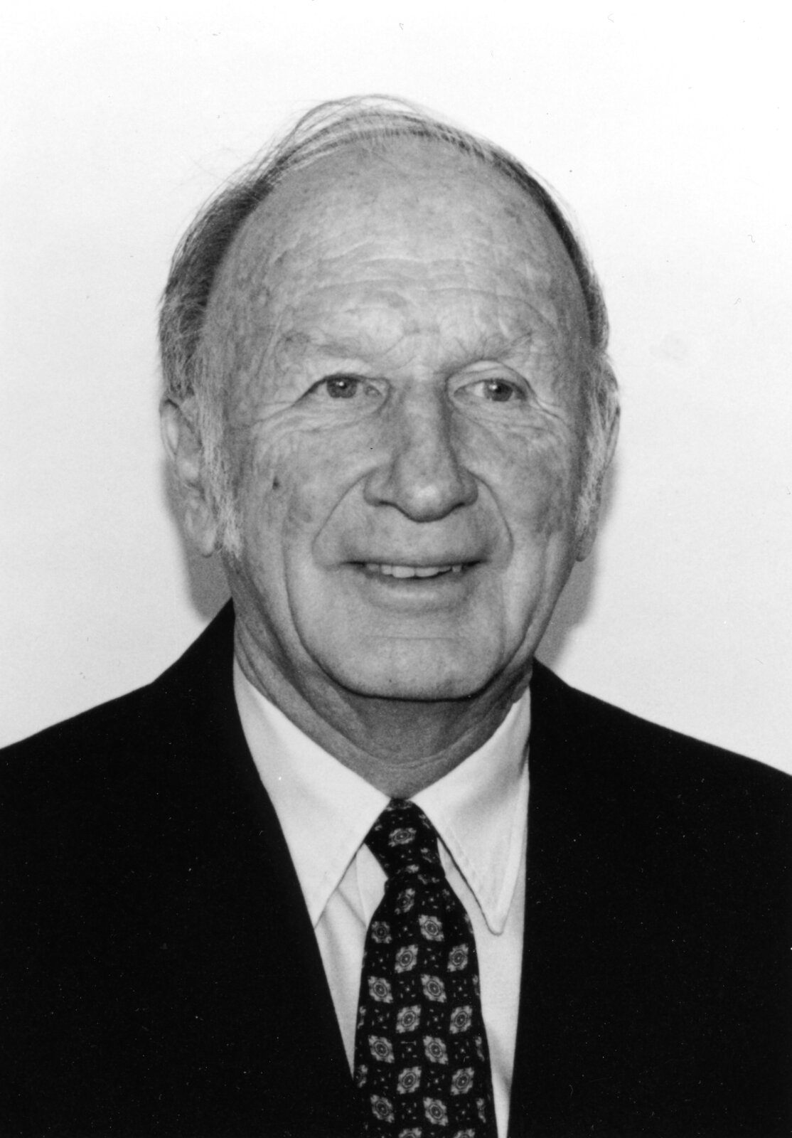
One day in the winter of 1961, in a small office in the Department of Meteorology of the Massachusetts Institute of Technology, a forty-three-year-old assistant professor named Edward Norton Lorenz typed a few numbers into the keyboard of a Royal McBee LGP-30 desktop computer, started a program, and walked out to get a cup of coffee. The machine – 113 vacuum tubes, 1450 diodes, a magnetic drum spinning at 3700 rpm, a Flexowriter typewriter for input and output, 60 multiplications per second – continued the run he had interrupted the previous afternoon. He had wanted to look more closely at a particular weather sequence the simulation had produced, so rather than re-run the program from the beginning, he had taken the values from the printout at some intermediate time and typed them back in as initial conditions for a continuation.
The numbers he typed were three decimal places long. The numbers in the machine’s drum memory were six decimal places long. The printer truncated.
When he came back from his coffee about an hour later, the new run agreed with the old for the first few simulated days, drifted noticeably from it for a few more, and then – with no warning and no obvious mechanical fault – diverged completely. The two solutions, started from numbers identical to a part in a thousand, ended up as unlike each other as any two random states of the model atmosphere he had been simulating.
He stared at the printout. He checked the punched paper tape. He restarted the program. The same thing happened again.
“At this point,” he later told Kerry Emanuel, in what is the closest thing on the record to a Lorenz Eureka quotation, “I became rather excited.”1
What he had found – and what it would take him two years to write up, fifteen years for the meteorological community to take seriously, and thirty-one years for the world’s operational forecast centres to engineer around – is now known as sensitive dependence on initial conditions, or in its popular form, the butterfly effect. The 1963 paper that resulted, “Deterministic nonperiodic flow,” in the Journal of the Atmospheric Sciences, did not stop the project of numerical weather prediction. It put a ceiling on it. It told von Neumann, Charney, Smagorinsky, Phillips, and every meteorologist after them that no matter how powerful the computer became and no matter how dense the observing network grew, weather prediction in the deterministic sense had an intrinsic horizon. Lorenz himself, in his 1969 follow-up in Tellus, would estimate that horizon at roughly two weeks for synoptic-scale forecasting on Earth’s atmosphere. The estimate has held up for sixty years.
This post is a portrait of the man who made that finding, of the desk-sized machine on which he made it, of the department that housed him for forty years without ever quite knowing what to do with him, and of the way his work eventually entered the operational forecasting bloodstream of every major weather centre on Earth.
Where Post 40 left off
The previous post in this series covered the seventeen-year directorship of Frederick Gale Shuman at the National Meteorological Center in Suitland, Maryland, from April 1964 to January 1981. The post’s central institutional finding was that an operational weather centre’s character can be set by one stubborn director with a long tenure: Shuman’s smoothing operator from 1957 was still in use four decades after he wrote it, the Limited Area Fine Mesh model he commissioned in 1969-1970 was still running operationally in 1994, and the Global Spectral Model he authorised five months before he retired ran in its descendant lineage until 12 June 2019.
That post was about the operational side of NWP – the side that signs the cheques, schedules the production runs, defends the model in front of the forecasters, and lives or dies by the verification statistics. This post is about the opposite pole: the theoretical side, the curiosity-driven academic department a few hundred miles north of Suitland on the banks of the Charles River, where one man working alone on a vacuum-tube machine quietly demonstrated that the operational programme had a horizon it could never cross. The two stories are the same story, told from opposite ends of the table. Shuman built up to the deterministic ceiling. Lorenz, in 1961, found the ceiling.
The man at the centre of this post is harder to write about than Shuman is. Shuman left an enormous documentary trail at NMC – internal memoranda, monthly office notes, the AMS award citations, the model verification logs. Lorenz left forty-three years of MIT teaching, a hundred peer-reviewed papers, three reserved-Yankee autobiographical statements (the 1991 Kyoto Prize lecture, the 1996 WMO interview, the 1993 Essence of Chaos), and a community of colleagues and students who all converge on the same description: gentle, modest, almost painfully shy, but warm and slyly funny with intimates, physically extraordinarily durable, in love with mountains and games and music and his family in roughly that order, and the kind of mathematician whose central insight came out of a coffee break rather than out of a research programme.
He has been described as a coyote. Kerry Emanuel told The Tech, the MIT student paper, that on a desert hike Lorenz “imitated coyotes” until actual coyotes responded.2 He has been described as having “the soul of an artist” – that was Jule Charney, who had the office two floors above his for twenty-five years and never wrote a paper with him.3 He has been described as a mountain goat, knowing every trail of the White Mountains of New Hampshire and the Rockies of Colorado. He has been described, by Physics Today on his death, as the man who, surveying the worldwide tributes after his obituary, would say only “I just don’t see what the fuss is about.”4
The fuss is real. Let us put the finding in its biography.
1. Hartford to Cambridge, 1917-1948
Edward Norton Lorenz was born in West Hartford, Connecticut, on 23 May 1917. His father was Edward Henry Lorenz, born in Hartford in 1882, a graduate of Hartford High School and Trinity College, and then of MIT in mechanical engineering (the MIT of that era was still on the downtown Boston side of the Charles, before the 1916 move to Cambridge). The father was small in stature, an excellent distance runner who held the MIT two-mile-run record, and “from him,” in Emanuel’s account, “his son acquired an early knowledge of science, particularly mathematics.” Father and son would compete on jigsaw puzzles and record their times on the inside covers of the boxes.5
A note worth making before going further: the brief I was working from when I started this series had Lorenz’s father down as a dentist. He was not. He was a mechanical engineer, an MIT graduate, and a recreational athlete. The error appears in some circulating popular sources but is contradicted by every primary biographical source – Lorenz’s own 1991 Kyoto Prize lecture, Emanuel’s 2011 NAS memoir, Tim Palmer’s 2009 Royal Society memoir, Britannica, MacTutor at St Andrews – which agree on the engineer attribution.
Lorenz’s mother was Grace Peloubet Norton, born in Auburndale, Massachusetts, in 1887, and a graduate of the University of Chicago. Her father, Lewis M. Norton, had developed the first course in chemical engineering at MIT in 1888 and died young, after which Grace’s mother had founded the home-economics department at the University of Chicago. Grace became a school teacher. She had a deep interest in games, particularly chess, which she passed on to her son. (Lorenz, Emanuel quotes, would say his mother “taught me more about life than anyone else.”)
So young Ed Lorenz grew up in a household with three generations of MIT connections on his father’s and his mother’s sides, with games as the central form of family play, and with summers at Waterville Valley in the White Mountains of New Hampshire (where his parents had met, married in 1916, and continued to summer for the rest of their lives). He had no documented siblings. (The brief I started from said “brothers”; no primary source mentions any.) The White Mountains were a fixture from the cradle; they would still be a fixture in his ninetieth year.
The mathematically precocious New England boyhood is the recurring portrait in every recollection of him. He read out house numbers from his go-cart to his mother before he could walk. After learning multiplication, he memorised all perfect squares between 1 and 10000. He learned the longhand method for square roots and cube roots. He was captain of his high-school and college chess teams. He kept his childhood jigsaw collection for life. At seven, he drew maps of imaginary places with inset enlargements. That same summer, visiting friends on a farm east of Hartford, he opened an atlas, saw illustrations of the planets, was struck by the rings of Saturn, and was launched into a lifelong love of astronomy. Aged eight, on a bitterly cold day in Hartford – the 24 January 1925 total solar eclipse, whose path of totality crossed Connecticut and southern New England – he watched shadow bands shimmering across fields of snow. He took up the violin at nine, decided he did not have the dexterity to make a pleasing sound from it, and switched to a lifelong passion for listening to concert music.
He was small for his age and a year younger than his classmates, which made him bad at team sports. He compensated by swimming underwater further than anyone else in the high school, and by hiking faster up White Mountain trails than anyone heavier. “Mountains and music were his greatest spare-time interests,” he would say later, by way of self-summary. They remained so for ninety years.
In 1934, aged seventeen, he entered Dartmouth College as a mathematics major. Of the seven hundred entering students that year, only seven would major in mathematics; Lorenz was one. He preferred the logical clarity of mathematics, in his own words, to any other subject he encountered, including history, physics, and geology. He graduated in 1938 with a Bachelor of Arts in mathematics.
He went on directly to Harvard University for graduate work in mathematics, “delighting,” as his own retrospective phrased it, “in being able to focus exclusively on math.” He studied group theory, set theory, and combinatorial topology under Saunders Mac Lane, Marshall Stone, and James Van Vleck (the last of whom would later win the Nobel Prize in physics). His master’s thesis advisor was George David Birkhoff, the most eminent American mathematician of his generation, best known for his proof of Poincaré’s Last Geometric Theorem and for the founding of modern ergodic theory. The thesis itself was on a problem in Riemannian geometry, not on dynamical systems. He took the AM in 1940 and continued for further doctoral work in mathematics at Harvard from 1940 to 1942.
The Birkhoff connection is one of the great curiosities of Lorenz’s intellectual genealogy. Through Birkhoff he was just one step removed from Poincaré and from the three-body problem – whose sensitive dependence on initial conditions Lorenz would, twenty years later, rediscover in atmospheric form and reformulate as modern chaos theory. There is no evidence Lorenz ever consciously read Poincaré in 1961. He stumbled onto the same phenomenon by his own route, on his own machine, in his own field.
Then came the war.
In early 1942, with the Harvard mathematics doctorate within reach but with the draft also within reach, Lorenz chose to enrol in an Army Air Corps weather-forecaster training programme. In March 1942 he became a cadet in an eight-month accelerated master’s programme at MIT, just across the Charles from Harvard. The faculty there was the first generation of academic meteorology in the United States: Hurd Willett, Henry Houghton, Bernard Haurwitz, working out of the department Carl-Gustaf Rossby had founded as a course in 1928. Lorenz emerged in 1943 with an SM in meteorology and a quiet resignation that the discipline he had been studying was meteorology and not the mathematics he had originally signed up for. He had been slow, he would say later, to appreciate the distinction.6
One specific frustration from those wartime cadet months would, twenty years later, turn out to define his life’s work. He had assumed naively, as a former mathematician, that the point of studying the dynamical equations of the atmosphere was to use them to make weather forecasts. The MIT faculty, he discovered, neither taught how to use the equations for forecasting nor told the cadets whether the equations could be used for forecasting at all. Some outstanding meteorologists at other universities, he was told, believed it was impossible. The gap between dynamical theory and forecasting practice would become, two decades later, the central problematic of his career.
After the cadet course he and four classmates were retained at MIT to teach the next year’s intake, which gave him time to take advanced classes. Then he shipped out: two months of tropical-meteorology training in Hawaii, then Saipan in October 1944, where he helped set up a weather-forecasting operation supporting the bombing of Japan. His specific role was chief of upper-level-winds forecasting. The observation density between Siberia and Saipan was wretched. The US aircrew were essentially the only observers, and as Lorenz would later remember dryly, “the pilots, to save time, would often simply repeat the forecast as the observation. This made for excellent forecast verification but hardly helped the forecasters make the next forecast.”
The weather operation moved to the Western Pacific in spring 1945 – to Guam, according to his colleague Patrick Suppes, or to Okinawa, according to Lorenz himself; the Battle of Okinawa did not end until mid-June 1945 and Suppes is probably right that the group moved to Guam first. Lorenz was appointed head of the upper-air section. The forecasting operation continued for several months after the surrender. He and the rest of his Weather Central unit were nominated, unsuccessfully, for a Bronze Star. The citation noted that the unit had “utilized scientific principles to adapt known techniques and to devise new techniques of analysis and forecasting in the institution of a successful combat weather forecasting service.”
When the war ended he faced a choice: return to Harvard to finish the mathematics doctorate, or stay in meteorology. He consulted Henry Houghton, the head of the MIT meteorology department. He chose meteorology. His own justification, given in his 1991 Kyoto Prize lecture, is worth quoting in full:
Mathematicians seem to have no difficulty in creating new concepts faster than the old ones become well understood, and there will undoubtedly always be many challenging problems to solve. Nevertheless, I believed that some of the unsolved meteorological problems were more fundamental, and I felt confident that I could contribute to some of their solutions.
He returned to MIT as a graduate student in meteorology. His doctoral advisor was James Murdoch Austin, a long-serving member of the department who specialised in storm dynamics. The brief I was working from when I started this series had Lorenz’s PhD advisor as Victor Starr, and the substitution is understandable – Starr was by far the more influential figure in Lorenz’s career – but it is a confusion. Austin supervised the doctorate. Starr came after.
The thesis was titled “A Method of Applying the Hydrodynamic and Thermodynamic Equations to Atmospheric Models,” and was a power-series-in-time expansion of the governing equations applied to storm motion. By the time Lorenz finished it, the Princeton team under John von Neumann was already mounting the rival approach – direct finite-difference numerical integration on the ENIAC. The ENIAC integration ran in March-April 1950 (the subject of the first post in this series on the founding of operational numerical weather prediction), and Lorenz’s series-expansion method was, by his own retrospective judgement, “more cumbersome than some others that were currently being developed” and was probably never used. But the thesis showed, as Emanuel notes, that Lorenz was “an innovative and independent thinker.” He received the ScD in 1948.
A few weeks later he married Jane Loban, who had been a research assistant in the MIT meteorology department where they had met. Jane was born in Dayton, Ohio in 1919, had grown up mostly in Cedar Falls, Iowa, and as a young woman had been a private pilot before she was old enough to drive a car. The path from aviation to meteorology was natural for her. They settled in Cambridge after the wedding, with an intermediate stretch some years later in Lexington, Massachusetts – where Ed sang in the town choir – and Cambridge again for their last years. (Some sources give Lincoln, Massachusetts; the correct town is Lexington.) They had three children – Nancy, Edward (called Ned), and Cheryl – and eventually four grandchildren. All three children inherited their parents’ love of puzzles and games, and all three became first-class downhill skiers. Lorenz’s own description of the family weekends, recorded in the Kyoto lecture: “Many of my winter weekends were spent taking one or all of them, usually with my wife as well, to some ski area north of Boston; this, of course, was just what I had hoped would happen.”
The pattern of his life was now set, and would not change for fifty years. MIT during the week. Family at home in Cambridge. Summers at Waterville Valley in the White Mountains and at the Chautauqua resort in Boulder, Colorado, where he and Jane would attend the student-orchestra concerts. Concert music. Chess at the MIT faculty club at lunch (sometimes against Norbert Wiener, who would play simultaneous games against several colleagues at once). Hiking. Skiing. And, as it turned out, the General Circulation Project.
2. Available potential energy: the paper that made his reputation
The brief lecture-room formula for Lorenz’s pre-chaos reputation is that he wrote one of the founding papers of modern atmospheric energetics in 1955. The full formula is more interesting and runs longer. The man who made him an atmospheric scientist was Victor Paul Starr.
Starr (1909-1976) had joined the MIT meteorology department after the war and was running what he called the MIT Planetary Circulation Project – sometimes called the General Circulation Project. The aim of the project was to understand, in quantitative observational terms, the energetics of the global atmosphere: what is the energy reservoir that drives the jet stream, where does mid-latitude eddy energy come from, why does the angular-momentum balance close the way it does. Rossby had pointed the way in the 1930s with the discovery of the long planetary wave; Starr’s contribution was the theory of negative viscosity – the surprising recognition that mid-latitude eddies systematically pump westerly momentum into the jet stream rather than diffusing it out, contrary to the standard turbulent-diffusion intuition.
Lorenz joined Starr’s project in 1948, immediately after finishing his ScD, as a research scientist. He stayed in the project intellectually for the next twenty-five years. The intellectual debt was profound and Lorenz did not hide it. From his 1991 Kyoto questionnaire response:
The things I remember best and cherish most, in looking back over my scientific career, are the almost daily conversations with Victor Starr during the more than twenty-five years that I worked with him, first as a protégé and then as a colleague.
The work for which Lorenz first earned a senior reputation in atmospheric science was the 1955 paper “Available potential energy and the maintenance of the general circulation,” Tellus 7, 157-167. The concept of available potential energy – the difference between the total potential energy of an atmospheric state and the minimum total potential energy attainable under any adiabatic redistribution of mass – had been introduced by Max Margules in 1903 for an isolated air mass; Lorenz generalised it to a planetary fluid in dynamical motion. The plain-language analogy worth pausing on, before any formula: imagine a tilted layer of cold air sitting underneath warm air. Gravity wants to flatten the layers; the tilt represents stored energy that could be released if the layers reorganised. Available potential energy is the maximum kinetic energy you could ever extract from such an atmosphere by letting it shake out adiabatically into its lowest-potential-energy configuration. It vanishes when the density stratification is horizontal and stable everywhere; otherwise it is positive and is approximately equal to a weighted vertical average of the horizontal variance of potential temperature.
Why this matters for weather: available potential energy is the reservoir that baroclinic instability taps to spin up extratropical cyclones. The Lorenz energy cycle (zonal-mean available potential energy goes to eddy available potential energy, eddy available potential energy goes to eddy kinetic energy, eddy kinetic energy goes to zonal-mean kinetic energy) became the standard diagnostic framework for general-circulation studies. Smagorinsky and Manabe – whose GFDL general circulation model was at that point still under construction – and the whole GFDL group adopted it. Two decades later, when the first generation of GCMs began producing serious long-integration output, the standard validation question for any new model was: does it give the right Lorenz energy cycle?
This was the paper that made Lorenz’s senior reputation. By 1963, when the chaos paper appeared, he was already a tenured full professor primarily on the strength of the 1955 APE paper, the 1967 WMO monograph The Nature and Theory of the General Circulation of the Atmosphere, and the energy-cycle diagnostics. He had been Assistant Professor since 1955 (Britannica gives 1954, MIT News and Wikipedia give 1955), Full Professor since 1962, and was a Fellow of the American Academy of Arts and Sciences from 1961. The chaos work, which would dominate his later historical reputation, was at the time of its 1963 publication an obscure curiosity buried in a journal article with a title – “Deterministic Nonperiodic Flow” – that the JAS editor had made him substitute for the more pointed “Deterministic Turbulence” he had wanted to use.7
3. The Statistical Forecasting Project and the LGP-30
The crucial context for what happens next is the one the popular accounts skip: Lorenz did not set out to discover chaos. He set out to disprove statistical weather forecasting.
In the late 1940s and 1950s a number of meteorologists believed that empirical linear-regression models fitted to past weather data could match the forecast skill of the new numerical-dynamical models coming out of Princeton. This view was bolstered, somewhat indirectly, by results of Norbert Wiener on linear prediction of stationary time series. The MIT Statistical Forecasting Project had been founded by Thomas Malone to investigate the question; Henry Houghton invited Lorenz to lead the project in 1948.
Lorenz did not believe linear regression could match dynamical forecasting. He set out to test it on irregular, non-periodic data – exactly the kind of data a linear model could not trivially fit. He needed a small dynamical system that would produce aperiodic output to feed into his linear-regression apparatus as a strawman. He started building such systems in the mid-1950s. By 1958 he had bought a machine to run them on.
The machine was a Royal McBee LGP-30.
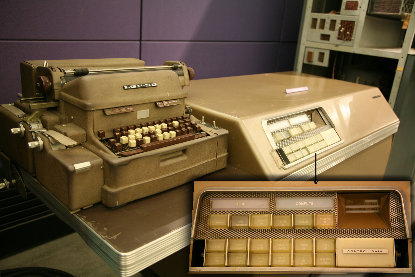
The LGP-30 – Librascope General Precision 30 – had been introduced in 1956 by Librascope and was sold in the United States by Royal Precision, a Royal McBee subsidiary. The hardware was modest even by the standards of late-1950s computing: about 113 vacuum tubes, around 1450 diodes, a magnetic drum spinning at 3700 revolutions per minute and holding 4096 31-bit words (the popular description as a “32-bit machine” is technically true but only 31 bits were data). Word access time was on the order of 0.26 milliseconds; inter-instruction access time was about 2.34 milliseconds, because every instruction had to wait for its successor address to come round under the read head before it could be executed. Arithmetic was bit-serial, fixed-point fractional. The headline arithmetic figure – the one that anchors this post’s title – is that the LGP-30 could carry out approximately 60 multiplications per second.8 (The looser “about one multiplication per second” that appears in some popular sources is wrong by roughly two orders of magnitude.) Programming was through paper tape, in hexadecimal plus the LGP-30’s idiosyncratic 16-character alphabet “0123456789fgjkqw.” The machine cost about 47000 1956 dollars. It weighed roughly 800 pounds and took up the floor space of a desk. James Gleick, who interviewed Lorenz extensively for the 1987 book Chaos, described it as having sounded “like a passing propeller plane.”
In 1958, when his LGP-30 arrived, Lorenz wrote that “Suddenly I realized that my desire to do things with numbers would be fulfilled.”9 He had a small dynamical system in his office that he could programme himself and that could run all night.
The actual programming on the LGP-30 was not done principally by Lorenz. Two women in turn did the bulk of it. Margaret Hamilton – the same Margaret Hamilton who would later lead the Apollo flight-software effort at MIT Draper Lab – arrived at MIT in the summer of 1959 with a fresh mathematics degree from Earlham College and no programming experience. She wrote and debugged the LGP-30 code for Lorenz’s models, editing binary instructions on paper tape with a pencil when necessary. She trained her replacement in the summer of 1961. The replacement was Ellen Fetter, a Mount Holyoke mathematics graduate of 1961. Fetter was the one running the program at the moment of the truncated-printout incident in winter 1961; she also produced the hand-plotted phase-space trajectories that became the famous strange-attractor figures of the 1963 paper.
It is worth flagging the women explicitly because the standard reading-public picture of Lorenz at the LGP-30 is of a single man typing in initial conditions, walking out for coffee, and finding chaos when he comes back. The man was Lorenz. The keyboard was Fetter’s. The reproducible day-to-day operation of the machine was Hamilton’s, and then Fetter’s. As Sokoler, Yoder, and Gabai recorded in their 2019 Quanta Magazine piece on the “hidden heroines of chaos,” Lorenz himself remarked late in his life that “every one of them would say that if this were going on today, they’d be a co-author.”
The model that ran on the LGP-30 from 1959 to 1961 was a 12-variable system of ordinary differential equations approximating the equations of motion of a rotating stratified fluid. The system was nonperiodic by design. Every Monday, Gleick records, “the other meteorologists would gather around with the graduate students, making bets on what Lorenz’s weather would do next.” The model became, in effect, the office sweepstake.
It was in this 12-variable model – not the famous 3-variable model that came later – that the truncation incident occurred.
4. The 1961 discovery and the 1963 paper
The discovery has been retold so many times that the specific provenance of its specific details deserves a careful read.
The qualitative description – that Lorenz typed three-digit numbers back into the machine which had stored six-digit numbers, walked away for coffee, came back to find the two runs had diverged completely – is given in Lorenz’s own retrospective writings, in the 1991 Kyoto lecture, in Emanuel’s 2011 memoir, and in The Essence of Chaos (1993). The specific digit pair – 0.506 typed, 0.506127 stored – comes from Gleick’s 1987 Chaos, derived from interviews with Lorenz. The qualitative version is the primary record; the specific digits are Gleick. They are widely repeated but I have not located them in Lorenz’s own written account. The 0.506 vs 0.506127 detail should always be attributed to Gleick.
The exact dating is similarly slightly soft. Gleick says “one day in the winter of 1961,” which is the most cautious statement supported by primary sources. Emanuel writes “at one point, in 1961.” The American Physical Society’s This Month in Physics History column for January 2003 places the discovery specifically in January 1961, but this appears to be APS editorial inference rather than a primary-source date. Stay with “winter 1961” unless and until a primary date can be pinned down.
What is documented beyond any ambiguity is what Lorenz did next. He realised that the divergence was not a bug. The machine, when given identical inputs, gave identical outputs. The inputs were not identical – the typed numbers and the drum-memory numbers differed in the fourth, fifth, and sixth decimal places – and the difference, miniscule though it was, had grown exponentially in time until it filled the entire state space of the model.
The implication was that the model – and by extension any sufficiently nonlinear deterministic atmospheric model, and by further extension the actual atmosphere – was exquisitely sensitive to its initial conditions. Forecasting from approximate initial conditions could give you only a finite window of skill no matter how accurate your dynamics were, because the inevitable initial-condition error would amplify until it swamped the signal.
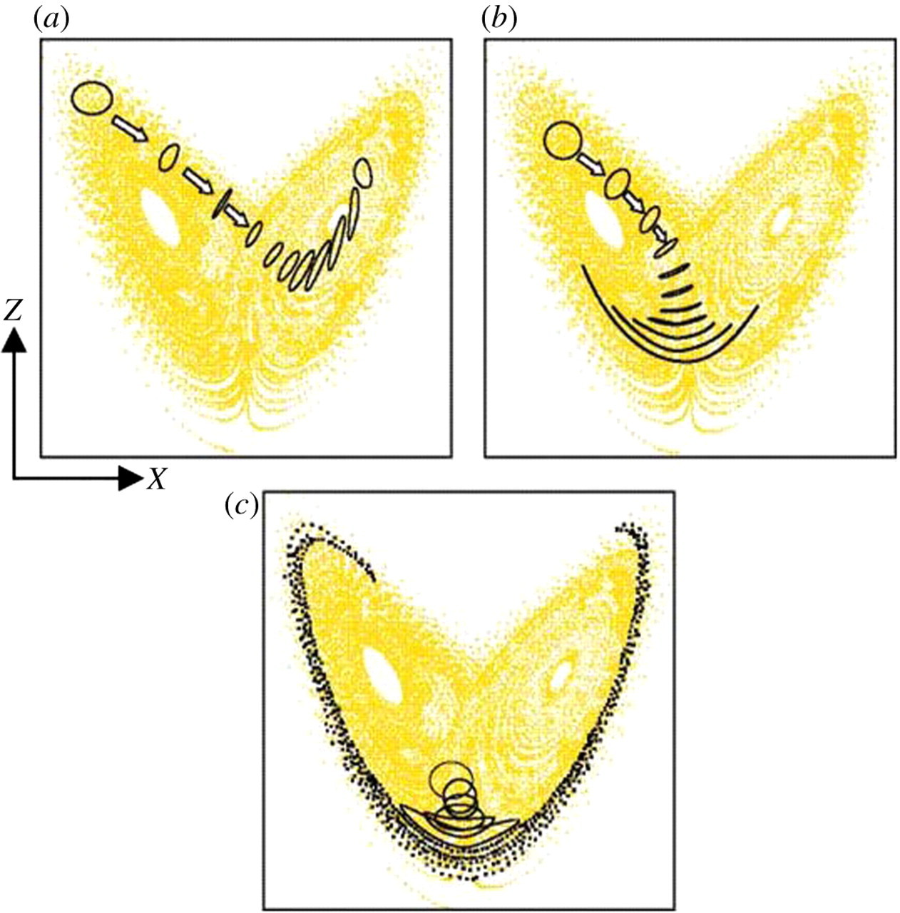
Lorenz spent the next two years working through the consequences. He wanted the simplest possible dynamical system that exhibited the same behaviour. Around 1962 he visited Barry Saltzman, then at the Travelers Research Center in Hartford, Connecticut. Saltzman had recently published a paper – “Finite amplitude free convection as an initial value problem - I,” J. Atmos. Sci. 19 (1962), 329-342 – which truncated a Rayleigh-Bénard convection problem (heated fluid in a horizontal layer, with the bottom warmer than the top) into seven coupled ordinary differential equations in the Fourier coefficients of the streamfunction and the temperature perturbation. In one of his runs, Saltzman noticed that four of the seven variables decayed to zero while the remaining three behaved aperiodically.
Saltzman did not pursue the aperiodicity. Lorenz, looking at Saltzman’s office floor full of printouts on that 1962 visit, saw what Saltzman had not pursued. As Emanuel describes it: “Ed noticed that in this particular solution, four of the seven variables settled down to zero and stayed that way. Thus he realized that there are chaotic solutions to a three-variable system; this became the celebrated Lorenz (1963,1) model.”
Lorenz was unfailingly generous about Saltzman in print. The 1963 paper cites Saltzman 1962 explicitly. The retrospective lectures and the Essence of Chaos repeat the citation. Saltzman, for his part, was gracious. The historical bookkeeping is straightforward: the convection equations are Saltzman’s; the reduction to three variables, the recognition that the three-variable system is chaotic, and the rigorous analysis of its attractor are Lorenz’s.
The system Lorenz arrived at, with its canonical parameters, is now known as the Lorenz equations. In the plain-language analogy: imagine a thin layer of fluid heated from below; the warm fluid wants to rise, the cool fluid wants to sink, and you get rolling convection cells like ridges in a saucepan of porridge on a stove. The three variables capture, respectively, how fast the rolls are turning, the temperature difference between rising and sinking branches, and the vertical bulge in the temperature profile that the convection creates. Then the equations themselves:
\(\dot{x} = \sigma(y - x)\) \(\dot{y} = rx - y - xz\) \(\dot{z} = xy - bz\)
with $\sigma$ (the Prandtl number, ratio of fluid viscosity to thermal diffusivity) typically set to 10, $r$ (the normalised Rayleigh number, basically how hard you are heating the fluid) typically set to 28, and $b$ (a geometric factor representing the aspect ratio of the convection rolls) typically set to 8/3. The critical Rayleigh value above which the system becomes chaotic is approximately $r_c \approx 24.74$; at $r = 28$ you are well above critical.
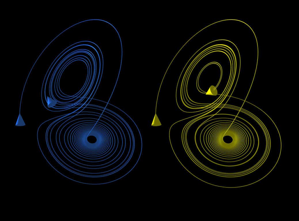
The 1963 paper, “Deterministic Nonperiodic Flow,” J. Atmos. Sci. 20 (1963), 130-141, did three things. First, it presented the three-variable system and showed that it had bounded solutions that never settled into a periodic orbit. Second, it demonstrated by direct numerical experiment on the LGP-30 that two solutions started from arbitrarily close initial conditions diverged from each other – exponentially – until they were as unlike as any two random states of the system. Third, and most subtly, it showed that the system’s long-term trajectory, traced out in the three-dimensional state space, lay on a set of zero volume but non-zero dimension – what we would now call a fractal attractor.
The geometric insight is worth dwelling on. Because the Lorenz system is dissipative – because the divergence of the flow in state space is negative, specifically equal to $-(\sigma + 1 + b) = -13.667$ – any finite volume in state space must shrink to zero as time goes on. And yet trajectories within the system diverge exponentially. Lorenz resolved the apparent paradox in the 1963 paper by arguing that the attractor must be a set of infinitely many surfaces, nested so finely that they appear to merge but never actually do:
It would seem, then, that the two surfaces merely appear to merge, and remain distinct surfaces. Following these surfaces along a path parallel to a trajectory, we see that each surface is really a pair of surfaces, so that, where they appear to merge, there are really four surfaces. Continuing this process for another circuit, we see that there are really eight surfaces, etc., and we finally conclude that there is an infinite complex of surfaces, each extremely close to one or the other of two merging surfaces.
This is the first description in the scientific literature of what would later be called a strange attractor (Ruelle and Takens 1971) or, more generally, a fractal (Mandelbrot 1975). Lorenz had described the object twelve years before it acquired its modern name and eight years before it acquired its modern technical theory.
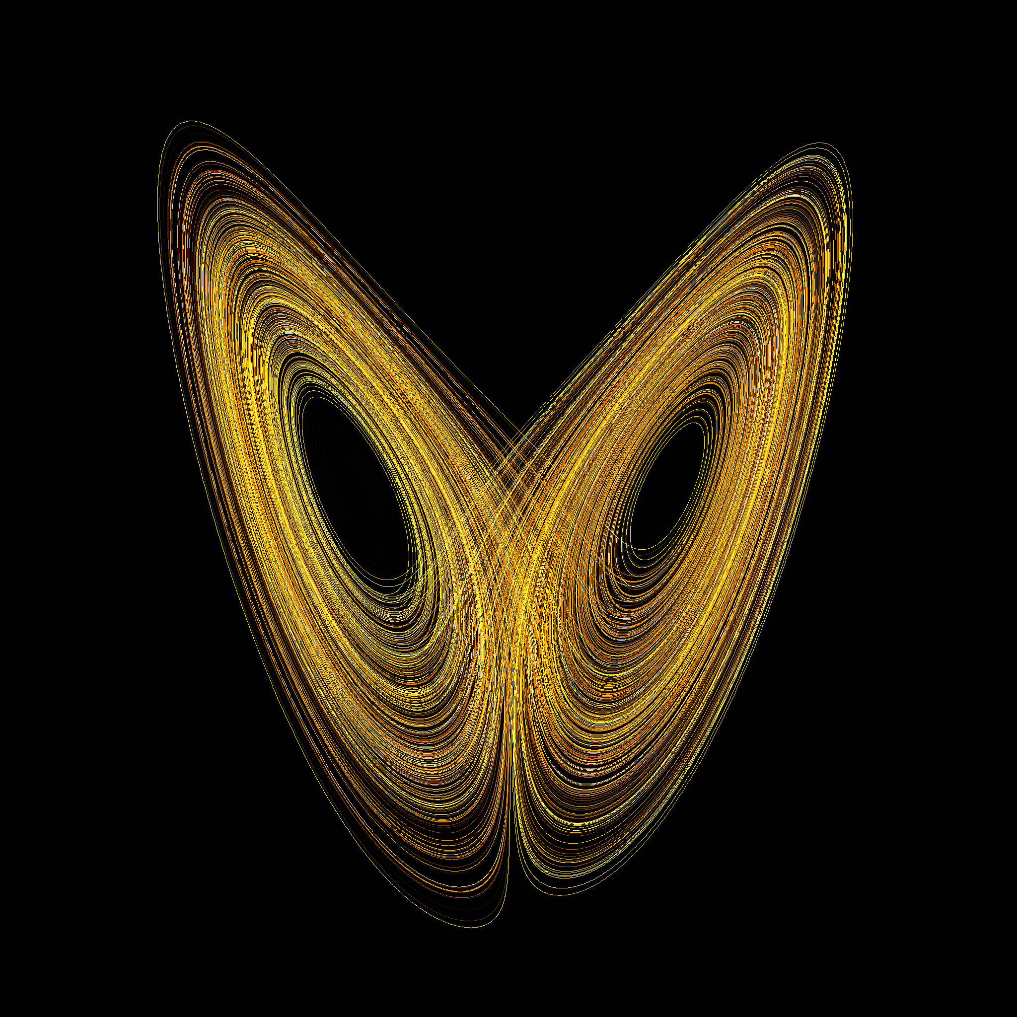
When Ellen Fetter hand-plotted the two-dimensional projections of the trajectory, they took on the shape that gave the attractor its informal name. The “butterfly” of the Lorenz attractor is its (x, z) projection. The (y, z) projection looks more like an owl’s face. Either way, the visual is the one most people now associate with chaos.
The companion result – the one that gave the post its working title – is what happens when you start two simulations from arbitrarily close initial conditions and let them run. Plain-language version: imagine two leaves dropped within a millimetre of each other into a turbulent stream. For the first few feet they drift downstream together. Then a small eddy pushes them apart by a centimetre, then the next eddy pushes them apart by a metre, then by ten metres, and within a hundred yards you have no hope of guessing where one will be by looking at the other.
This sensitive dependence had a prior life in Lorenz’s own writing, in his other 1963 paper – “The mechanics of vacillation,” J. Atmos. Sci. 20, 448-464. That paper contains what is now the canonical Lorenz statement of the butterfly idea in seagull form:
One meteorologist remarked that if the theory were correct, one flap of a sea gull’s wings would be enough to alter the course of the weather forever. The controversy has not yet been settled, but the most recent evidence seems to favor the gulls.
The seagull is the original avian metaphor for sensitive dependence. The butterfly came later, and as the next section will show, did not come from Lorenz at all.
5. The slow reception, 1963-1978
If the 1963 paper is so important, why did nobody read it for fifteen years?
The citation history is unambiguous. Physics Today’s 2013 fiftieth-anniversary essay reports fewer than twenty citations of “Deterministic Nonperiodic Flow” in the meteorological literature in its first twelve years. Lorenz did get the Carl-Gustaf Rossby Research Medal in 1969 – the highest scientific honour of the American Meteorological Society – but it was awarded principally for his work on available potential energy and on the general circulation, not for chaos. He was elected to the National Academy of Sciences in 1975, again on cumulative merit rather than on the 1963 paper alone.
The reasons the meteorological community ignored the chaos result for fifteen years are reasonably clear and worth separating out.
Different language. The mathematical apparatus of Poincaré-Hadamard-Birkhoff dynamical-systems theory – measure theory, hyperbolic dynamics, ergodic theorems – lived in pure mathematics departments. Meteorologists in 1963 thought in partial differential equations and finite-difference grids. The interface between the two communities was thin. Lorenz himself, who had a Harvard mathematics graduate education and George Birkhoff as his master’s advisor, was unusually bilingual; very few of his readers were.
Different problem. The classical chaos literature – Poincaré’s 1889 three-body essay, Hadamard’s 1898 geodesics on negatively curved surfaces, Birkhoff’s 1931 ergodic theorem – was about Hamiltonian (conservative, volume-preserving) systems. The atmosphere is dissipative (volume-contracting in state space because friction and radiation drain energy out of it). Strange attractors are phenomena of dissipative systems and had no analogue in Hamiltonian dynamics. Even Poincaré’s homoclinic tangle is not the same geometric object as Lorenz’s attractor. So even meteorologists who had read Poincaré (and there were few) would not have recognised the family resemblance.
The optimism of NWP. From Richardson’s 1922 Weather Prediction by Numerical Process through von Neumann’s 1950 ENIAC experiments and Charney’s first operational forecasts at JNWPU in 1955, the prevailing institutional view was that better physics and faster computers would buy unlimited forecast skill. Von Neumann actively believed that weather control was feasible. As Gleick recorded, von Neumann “gave breathtaking talks about his plans” for cloud-seeding and weather modification on continental scales. Nothing in this optimistic institutional project pointed researchers toward ergodic theory or sensitive dependence. Lorenz’s 1963 result was an unwelcome correction to a programme that was, at that exact moment, getting its first major operational deliverables.
Lorenz’s own modesty. He did not push the result. He published it once, gave a few seminar talks, and went back to working on the general circulation. He did not give interviews, did not lobby. The paper sat in the literature waiting to be found.
It was the mathematicians, not the meteorologists, who eventually found it.
The pipeline went roughly like this. Stephen Smale at Berkeley and his students were building up the geometric theory of differentiable dynamical systems through the 1960s, working independently of Lorenz on hyperbolic dynamics, the horseshoe map, and structural stability. David Ruelle and Floris Takens in 1971, in “On the nature of turbulence” (Commun. Math. Phys. 20, 167-192), coined the term strange attractor for chaotic invariant sets of dissipative systems. Ruelle and Takens did not cite Lorenz in their 1971 paper – a fact that Ruelle later acknowledged as an oversight; Lorenz’s 1963 work had, as Ruelle put it, been “unfortunately overlooked.” It was James Yorke (Maryland) who is conventionally credited with bringing Lorenz’s equations to Smale’s circle of dynamicists around 1972, and Tien-Yien Li and James Yorke in 1975 published “Period three implies chaos” in the American Mathematical Monthly, which coined the word chaos in its modern technical sense.
By the mid-1970s the term “Lorenz attractor” was current among physicists and applied mathematicians. Otto Rössler in 1976 published an even simpler chaotic attractor with only one quadratic nonlinearity, explicitly modelled on Lorenz’s. Mitchell Feigenbaum’s discovery of the universal scaling constants of the period-doubling route to chaos came in 1978. By the early 1980s, chaos was a recognised research field, with its own journals, its own conferences, and its own undergraduate textbooks. The 1963 paper had finally been read.
The book that brought the story to the general public, and that turned “butterfly effect” into a household phrase, was James Gleick’s Chaos: Making a New Science, published by Viking in 1987. Gleick had interviewed Lorenz extensively. Chapter 1 of the book – titled “The Butterfly Effect” – is essentially a retelling of the LGP-30 truncation incident with full novelistic flair. Gleick’s account is now the primary popular source for many of the recollected details, including the 0.506 / 0.506127 digit pair.
By Lorenz’s seventy-fifth year, in May 1992, the citation count of the 1963 paper had exploded; chaos was a standard part of physics curricula; he was acquiring honorary degrees at the rate of one a year; and his 1969 Tellus paper – which, as the next section will argue, is more important for operational meteorology than the 1963 paper is – was about to be operationalised at two of the world’s largest forecasting centres simultaneously.
6. The 1969 paper: the predictability horizon
The 1963 paper showed that some deterministic systems are chaotic. The interesting question for forecasters is whether the atmosphere is chaotic in a way that matters operationally. To answer that, Lorenz needed a different model.
The three-variable system of 1963 has, by construction, three degrees of freedom. The actual atmosphere has something like $10^{20}$ molecular degrees of freedom, or, if you count on the scales meteorologists care about, on the order of $10^7$ grid-cell degrees of freedom in a high-resolution operational model. The interesting question for predictability of the atmosphere is therefore: how does error behave in a high-dimensional flow with a continuous spectrum of scales of motion?
This is the question Lorenz addressed in the 1969 paper “The predictability of a flow which possesses many scales of motion,” Tellus 21, 289-307.
The setup of the 1969 paper is a two-dimensional barotropic vorticity equation on a doubly-periodic domain. Plain-language version: think of a thin, horizontal sheet of fluid stirred so vigorously that it has eddies on every scale you can think of, from the size of a teacup to the size of an ocean basin, with the energy distributed across scales in a particular way. Lorenz decomposes this spectrum into discrete “scale bands,” each spanning a factor-of-two range in spatial wavenumber. He then derives, with a closure assumption about how energy transfers between scales, a closed system of evolution equations for the ensemble-mean energy of the error in each scale band. The error is the difference between the true atmospheric state and a forecast that started from an imperfect initial condition.
The key result depends on the slope of the background energy spectrum – on how energy is partitioned across the size scales of the eddies.
For a $k^{-5/3}$ Kolmogorov spectrum (the inertial-range spectrum of three-dimensional turbulence), Lorenz showed that the predictability horizon is finite even in the limit of vanishing initial error. Reducing the initial error by an arbitrary factor does not buy you an arbitrary amount of extra forecast skill; the time-to-saturation grows only logarithmically with the inverse initial error. Practically: if your initial-condition error halves, you gain a fixed additional amount of forecast time – not a doubling. There is a wall.
For a $k^{-3}$ spectrum (a steeper spectrum, which matches the atmospheric synoptic-scale energy distribution observed in radiosonde data) the predictability horizon is asymptotically infinite as initial error tends to zero – but only logarithmically slowly. In practice, with realistic initial-condition uncertainty, the horizon is again roughly finite.
In both cases what happens is an upscale error cascade. Errors that start out localised at small scales saturate quickly (their available variance fills up in hours), and then bleed up into the next-larger scale band, saturating that band after a longer time, and so on. The total time for a small-scale error to propagate from the smallest resolved scale up to synoptic scales is the predictability horizon for synoptic-scale forecasting.
Lorenz’s own numerical estimates, given in the 1969 paper, are:
- Cumulus-scale errors (order one kilometre, individual cloud or thermal): saturate in about one hour.
- Mesoscale errors (order ten to a hundred kilometres, a thunderstorm system): saturate in a few hours.
- Synoptic-scale errors (order one thousand kilometres, a continental weather system): saturate in a few days.
- Planetary-scale errors (order ten thousand kilometres): saturate in a few weeks.
The total upscale cascade time for synoptic-scale forecasting, on Lorenz’s parameter choices, came out at roughly two weeks. This is the origin of the “two-week limit” that has been operational-meteorology folklore ever since.
It is worth stating clearly that the two-week number is not a theorem. It depends on the assumed energy-spectrum slope and on the assumed error-doubling time at the smallest scales. Recent papers (Zhang and others, 2019; Shen and Pielke and others, 2024) have argued that the original two-week estimate combined Lorenz’s 1969 cascade model with a small-scale doubling time of approximately five days drawn from the Mintz-Arakawa GCM then circulating at UCLA. The GFDL spectral model of Smagorinsky and Manabe, used independently for predictability experiments, gave a doubling time of about ten days for the first thirty days of integration, dropping to six or seven days for the second thirty days as the model output became more aperiodic. So the precise number (“two weeks,” “ten days,” “fourteen days”) moves around in the literature; the qualitative result – a finite deterministic-forecast horizon in the range one to three weeks, set by intrinsic upscale error cascade and not by computing power or observation density – has not budged in sixty years.
The reason 1969 matters more than 1963 for operational weather prediction is exactly this. The 1963 paper shows that there exist three-variable systems that are chaotic. The 1969 paper shows that the atmosphere itself is chaotic in a way that imposes a hard ceiling on deterministic forecast skill, and that you cannot beat that ceiling by buying a faster computer or by launching more radiosondes. The 1969 paper is the theoretical foundation on which all of ensemble forecasting was eventually built.
A follow-up in 1982 – “Atmospheric predictability experiments with a large numerical model,” Tellus 34, 505-513 – did the operational comparison. By 1982 Lorenz had access to actual ECMWF forecasts. He compared, over a hundred-day period, the operational forecasts at different lead times against each other and against the verifying analyses. The methodology: take the day-D analysis, compare it to the (D-1)-day forecast valid for day D, the (D-2)-day forecast, etc. From the differences, you can extract both an upper bound on predictability (perfect-model, small-initial-error growth rate) and a lower bound (the operational skill of the day).
Lorenz’s 1982 finding, in Emanuel’s summary: “errors in the pressure field roughly 5 km above the surface doubled in about 2.5 days.” He warned, presciently, that as model resolution improved the doubling time would shrink, because higher-resolution models would resolve faster-growing small-scale errors. This implied an asymptotic plateau in operational forecast skill rather than a continuing increase – which is exactly the curve that Bauer, Thorpe and Brunet would document thirty-three years later, in their 2015 Nature paper “The quiet revolution of numerical weather prediction,” when the curve of operational skill at the major centres had flattened around day 9-10.
The 1982 paper also gave a hopeful estimate: “predictions at least ten days ahead as skilful as predictions made seven days ahead appear to be possible.” This was the theoretical headroom that ECMWF would eventually realise in the 2000s and 2010s – not by improving deterministic models per se, but by building the ensemble systems that the 1969 paper had implied were needed.
7. The butterfly enters folklore
The 1969 Tellus paper is, mathematically, where Lorenz spelled out the predictability argument that mattered for operations. But the world remembers it through the 1972 Washington DC talk, and the 1972 talk had a title that Lorenz himself did not write.
The talk was given on 29 December 1972 at the 139th meeting of the American Association for the Advancement of Science in Washington, in the Section on Environmental Sciences. The session convener was a meteorologist named Philip Merilees, then at NCAR. Lorenz had agreed to speak. He had not, however, sent Merilees a title in time for the printed programme. Merilees needed to put something in the programme. He could not reach Lorenz. So Merilees made up a title. The title he made up was:
Predictability: Does the flap of a butterfly’s wings in Brazil set off a tornado in Texas?
This is the origin of the “butterfly effect” as a phrase. Three observations are worth making about it.
First: the title was Merilees, not Lorenz. The Wikipedia Butterfly effect article quotes Lorenz himself on this point. Merilees concocted the title to fill the printed slot; Lorenz used the title when he delivered the talk because it was already in the programme.
Second: the butterfly, as opposed to the seagull of the 1963 paper, may have been introduced into the meteorological discourse not by Lorenz or by Merilees but by Joseph Smagorinsky. Smagorinsky’s 1969 BAMS article “Problems and promises of deterministic extended range forecasting” used the butterfly metaphor specifically, three years before Merilees needed a title. So the butterfly may have travelled from Smagorinsky’s 1969 BAMS article into Merilees’ programme entry into the talk title into Lorenz’s delivered text. The lineage is tangled and not entirely settlable.
Third: the concept of sensitive dependence is Lorenz, and has an even older ancestry. Emanuel’s NAS memoir traces the literary lineage of small-creature-changes-the-weather all the way back to William S. Franklin’s 1898 review (in Phys. Rev. 6, 170-175) of Pierre Duhem:
Long range detailed weather prediction is therefore impossible, and the only detailed prediction which is possible is the inference of the ultimate trend and character of a storm from observations of its early stages; and the accuracy of this prediction is subject to the condition that the flight of a grasshopper in Montana may turn a storm aside from Philadelphia to New York!
So before Lorenz’s seagull and Smagorinsky/Merilees’ butterfly, there was Franklin’s grasshopper. The trope predates Lorenz by sixty-five years.
Sometimes, on internet forums and in popular essays, the claim circulates that the 1972 talk was never actually delivered – that the title was published in the programme but the talk itself was abstracted or cancelled. This claim is wrong. The MIT Technology Review’s 2011 essay “When the butterfly effect took flight” treats the talk as delivered. Roger Pielke’s Honest Broker substack treats the talk as delivered. The text of the talk – about 1100 words – circulated in photocopies for decades and was reprinted as Appendix 1 of Lorenz’s 1993 book The Essence of Chaos. It was delivered.
The content of the talk itself is essentially a summary of the 1969 Tellus paper for a general audience, framed by two opening propositions that get at the conceptual core:
If a single flap of a butterfly’s wing can be instrumental in generating a tornado, so also can all the previous and subsequent flaps of its wings, as can the flaps of the wings of millions of other butterflies, not to mention the activities of innumerable more powerful creatures, including our own species.
If the flap of a butterfly’s wings can be instrumental in generating a tornado, it can equally well be instrumental in preventing a tornado.
The technical reformulation – “is the behaviour of the atmosphere unstable with respect to perturbations of small amplitude?” – recovers the seriousness. The four findings are essentially a layman’s version of the 1969 paper: coarse-structure errors double in about three days; fine-structure errors double in hours or less; fine-structure errors cascade upscale into coarse structure and cap useful prediction regardless of how dense the fine-scale observation network gets; temporally averaged quantities like weekly mean temperature may still be predictable beyond the deterministic limit. The last point is the seed of what we now call sub-seasonal to seasonal (S2S) prediction.
The closing line, with a nod to the Global Atmospheric Research Programme that Charney was then chairing, is the most-quoted sentence in the talk:
It is to the ultimate purpose of making not exact forecasts but the best forecasts which the atmosphere is willing to have us make that the Global Atmospheric Research Program is dedicated.
This is the only place in Lorenz’s published work where the operational implication of chaos is spelled out for a general audience. The project of weather forecasting, as Lorenz tells it here, is not the project of perfect prediction. It is the project of producing the best forecasts the atmosphere is willing to let us have. That formulation, and the talk’s borrowed title, would in 1987 be picked up by James Gleick, woven into Chapter 1 of Chaos, and broadcast to a worldwide reading public. By 1990 every American with a popular-science bookshelf knew the phrase “butterfly effect.” The seagull had been forgotten.
8. Charney down the hall: MIT 1956-1981
Lorenz’s working environment at MIT was a peculiar one. He had been at the department continuously since the 1942 cadet course, with one visiting year at UCLA in 1953-54. He became Assistant Professor in 1955, Full Professor in 1962, and Department Head in 1977. He worked alone, or with one computational assistant, on a vacuum-tube desktop machine that he programmed himself. His doors were said to open silently, and Emanuel records that “generations of students and colleagues at MIT will remember many occasions when Ed would appear silently in their office, as if by magic, and enthuse over some feature of the current weather map.” The forecasting interest, born in the Army Air Corps, never left him.
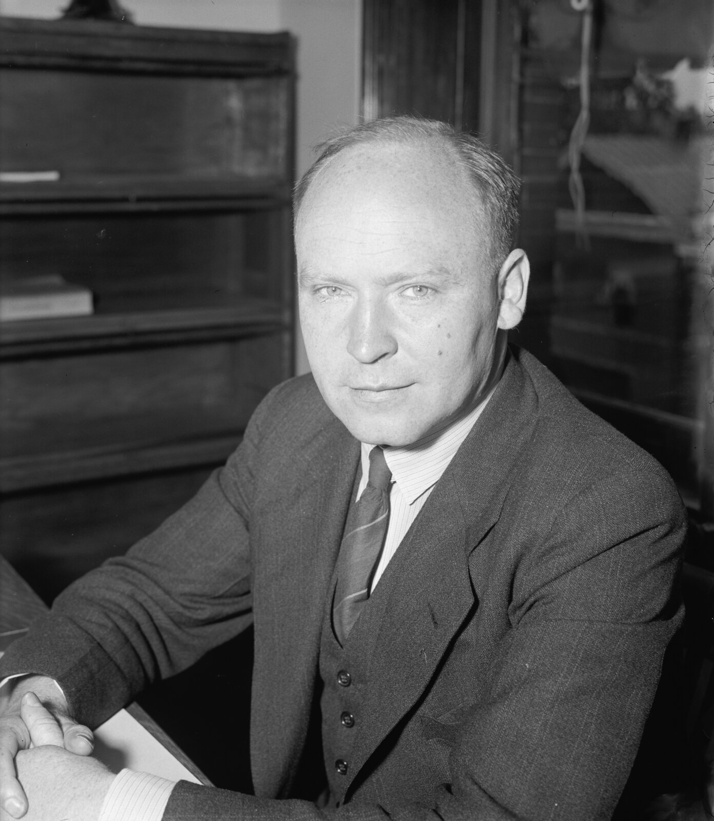
Two floors above him, after 1964, sat Jule Gregory Charney.
Charney had moved from the Institute for Advanced Study at Princeton to MIT in 1956 after the IAS Electronic Computer Project was wound down (von Neumann had been diagnosed with cancer in summer 1955 and died in February 1957). The story most repeated in MIT meteorology folklore is that Charney accepted the senior chair Houghton offered him on two conditions: that Norman Phillips – author of the first general circulation model integration, 1956 – come with him as a package deal, and that Lorenz be promoted from research scientist to assistant professor. Houghton agreed to both, and within a few years the MIT meteorology department housed Charney (quasi-geostrophic theory, baroclinic instability, ENIAC veteran), Phillips (first GCM), Lorenz (energetics, then chaos), Starr (general circulation observational programme), and Houghton (cloud physics, department head). It was, by the standards of any decade in atmospheric science, an absurdly strong line-up.
Lorenz and Charney were colleagues for twenty-five years – from Charney’s arrival in 1956 to his death from lung cancer on 16 June 1981. They shared MIT meteorology, they shared the Green Building after 1964, they served together on the 1966 NAS panel on predictability that produced The Feasibility of a Global Observation and Analysis Experiment. And in twenty-five years they never co-authored a single peer-reviewed paper.
That has to be one of the more remarkable facts in the history of the discipline. Two of the most important figures in twentieth-century atmospheric science, in the same department, on the same corridor, for a quarter of a century, with friendly relations and overlapping intellectual interests, never wrote a paper together. The likely explanation is style: Charney worked in large collaborative projects (the ENIAC team, the IAS group, GARP, the 1979 CO2 panel that would become known as the Charney Report), while Lorenz worked alone or with a single computational assistant (Hamilton, Fetter). Their intellectual territories overlapped only at the edges – Charney on baroclinic instability and large-scale dynamics, Lorenz on energetics and predictability of low-order systems.
Their relationship in person was warm. Charney is the one who famously described Lorenz as “a man with the soul of an artist.” David Randall, who was Charney’s student in the 1970s, said at the 2018 MIT Chaos and Climate symposium that “being in the room with Charney was like being in the room with a tiger, a very friendly tiger.” The complementarity is the point. Charney built the deterministic NWP programme. Lorenz quietly demonstrated its fundamental limits. There is no record in the literature of public friction between them on the predictability question – by the late 1960s Charney had accepted Lorenz’s results and incorporated them into his own GARP-era thinking. The 1966 NAS predictability panel that Charney chaired (and Lorenz, Mintz, Arakawa, Smagorinsky, and Leith served on) established the empirical five-day error-doubling time in GCMs and effectively codified the two-week deterministic horizon as official US scientific policy.
Around them on the corridor were a striking cast of supporting figures. Norman Phillips was research associate, then associate professor, then full professor, and finally Department Head 1970-1974. He left MIT in 1974 to become Principal Scientist at the National Meteorological Center in Suitland, an institutional move that bridged the academic and operational worlds for a generation; he stayed at NMC until 1988 and wrote Charney’s NAS biographical memoir in 1995. Fred Sanders – the synoptic-meteorology specialist, who would coin the term “bomb” for explosively deepening extratropical cyclones in his 1980 paper – was a junior colleague who taught practical map analysis to grad students alongside the dynamical theory they got from Charney and Phillips. Reginald Newell was the global-transport and climate-observations specialist; Erik Mollo-Christensen – a Norwegian Buchenwald survivor who came to MIT in 1946 – worked on turbulence and on ocean tides. Henry Stommel, the most important physical oceanographer of his generation, joined the MIT Department of Meteorology in 1963 from Harvard and shared the world with Lorenz until 1978; the two of them would share the 1983 Crafoord Prize.
And after 1981, when Charney died, the most important figure on the corridor for Lorenz’s late life would be Kerry Emanuel – a hurricane theorist who had just finished his PhD with Charney and would become, over the next quarter-century, the most authoritative chronicler of Lorenz’s intellectual style.

9. The personality, the family, and the mountains
There is a temptation, in writing about a quiet career, to deal with the personality in a couple of paragraphs and move on. Lorenz’s personality is the more rewarding thing to dwell on, partly because every colleague who wrote about him returned to the same themes, and partly because the personality and the science are obviously of a piece.
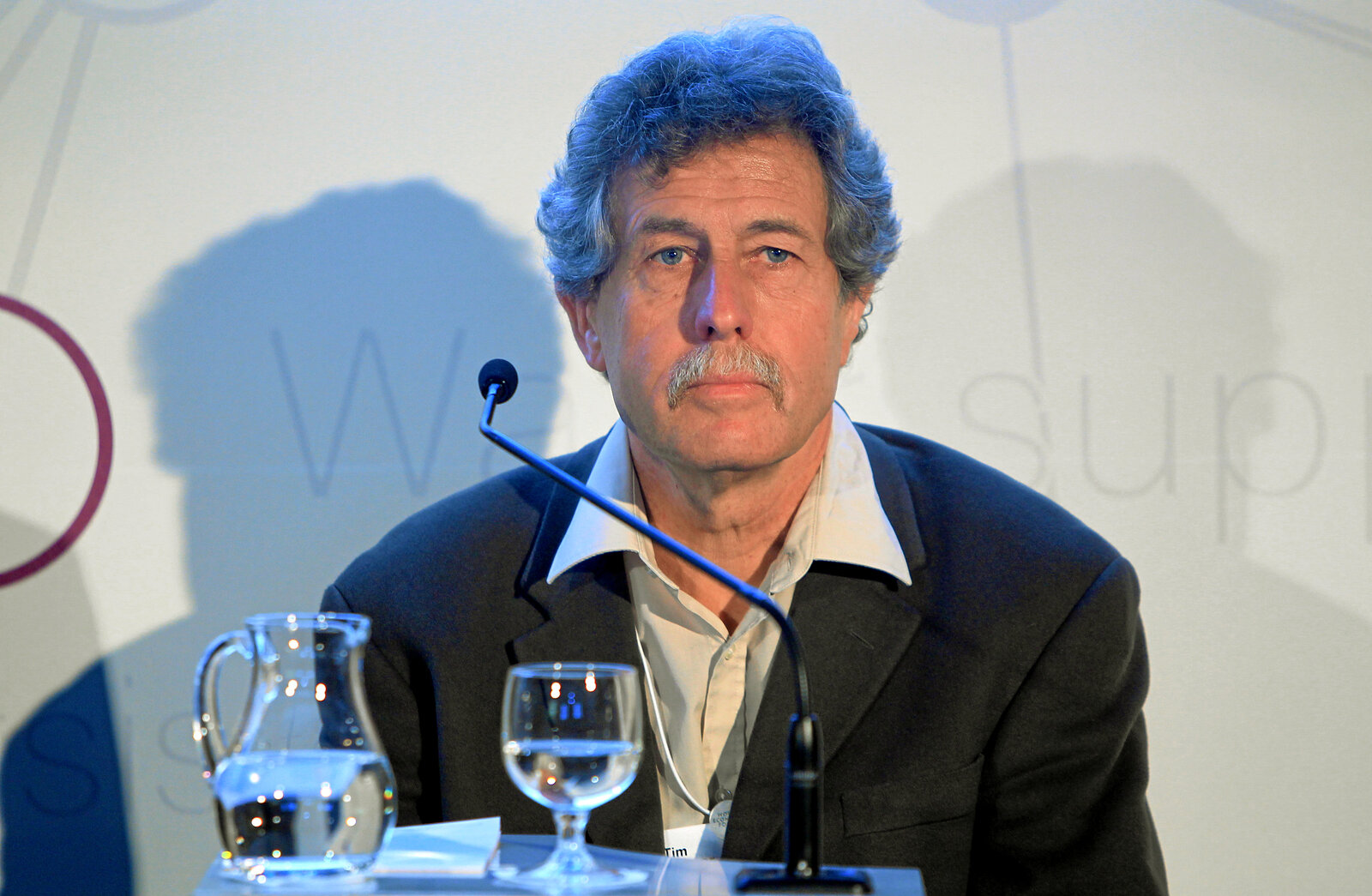
The dominant theme is reserve. Emanuel: “Those of us privileged to have known Ed Lorenz will remember him as a gentle, quiet soul, almost painfully shy and modest to a fault.” The Physics Today obituary used “extremely modest” and imagined Lorenz, on seeing the worldwide tributes after his death, saying simply “I just don’t see what the fuss is about.” Tim Palmer, who wrote the Royal Society biographical memoir in 2009 (the memoir itself is, sadly, paywalled and could not be retrieved for this post; the relevant passages are quoted by Emanuel), used the same words: shy, modest, deeply uninterested in self-promotion.
But the reserve was not coldness. The colleagues who got past it – and there were several generations of them – reported a warmer figure than the surface suggested. From Emanuel again: “But engage him on a favorite topic – a fine point in atmospheric or dynamical systems theory, the virtues of a particular mountain trail, or anything to do with his extended family – and with a twinkle of his bright blue eyes he would come to life; at such times one always felt as if he were inwardly smiling at life.”
The coyote story is the one I keep coming back to. The Tech, the MIT student paper, in its 18 April 2008 obituary, preserved an Emanuel anecdote that the more formal obituaries leave out: on a desert hike, Lorenz had imitated coyotes until actual coyotes responded. The image – a quiet New Englander, in late middle age, calling back-and-forth with the desert – is the one I think captures him best. The man who heard the desert and answered. The mathematician who, on coming back from coffee one afternoon in 1961, saw the printout and quietly became “rather excited,” and then went home for dinner.
The outdoor habit was extreme. Emanuel called him “like a mountain goat” and said he knew “every trail” in both the White Mountains of New Hampshire and the Rockies of Colorado. The Lorenz Center’s photo archive on its memorial page records hikes at the Flatirons near Boulder, in the Whites, on Mount Battie in Camden, Maine. The Times of London obituary described him as “a very keen outdoorsman who enjoyed hiking and cross-country skiing until well into old age.” Multiple sources confirm he was still skiing in his eighties and “managed to continue most of his regular activities until only a few weeks before his death.”
Devotion to family was the matching habit. He was, in Emanuel’s phrase, “old-fashioned” in his “sense of chivalry toward Jane.” When he visited colleagues at home he would arrive with mathematics-based toys for the children. He taught generations of MIT graduate students, won the graduate-students’ best-teacher award repeatedly, and was a fixture of the Lexington town choir while the family was based there. From the late 1990s, when Jane began to suffer “a series of debilitating illnesses,” he set his research aside and devoted himself to her care. Jane died in late 2001.
After Jane’s death he went back to research. He published roughly nine further papers in the seven years before his own death in 2008 – including, in 1991, “Dimension of weather and climate attractors” in Nature; in 1993, the book The Essence of Chaos; in 1995, his presentation at the ECMWF Predictability Seminar in Reading that introduced what is now known as the Lorenz 96 model; in 1998, the adaptive-sampling paper “Optimal sites for supplementary weather observations” with Emanuel; in 2006, “Regimes in simple systems”; and – published posthumously in 2008 – “Compound windows of the Hénon map” in Physica D 237, on whose proofs he was working a few days before he died. The Lorenz 96 model, a one-dimensional chain of $K$ ordinary differential equations with nearest-neighbour quadratic coupling and a constant forcing term, has become the workhorse of modern ensemble data-assimilation research. It is to predictability research what the Ising model is to statistical mechanics: a small, controllable, generic test bed.
There is one more autobiographical fragment worth quoting, partly because it is characteristically Lorenzian in its construction and partly because it bears on the Pascal-Birkhoff philosophical lineage of his mathematics. From The Essence of Chaos, on free will:
We must wholeheartedly believe in free will. If free will is a reality, we shall have made the correct choice. If it is not, we shall still not have made an incorrect choice, because we shall not have made any choice at all, not having a free will to do so.
Emanuel calls this “characteristic Lorenzian fashion” and notes that it is Pascal’s wager applied to determinism. The construction is what gives it away: the man who proved that small initial-condition uncertainties cascade into total ignorance was the same man who wrote epistemological aphorisms in the form of two-clause hypothetical syllogisms.
10. The 1992 operational triumph
When Lorenz turned seventy-five on 23 May 1992, the operational consequences of his work were about to land at two of the world’s largest forecasting centres almost simultaneously.
The operational launches were:
| Centre | System | Operational date | Lead architects | Initial-perturbation method |
|---|---|---|---|---|
| ECMWF Reading | Ensemble Prediction System (EPS) | late November 1992 | T. N. Palmer, F. Molteni, R. Buizza | Singular vectors |
| NMC/NCEP Washington | Global ensemble forecast system | 7 December 1992 | E. Kalnay, Z. Toth | Bred vectors (breeding of growing modes) |
Both centres had been working on initial-perturbation methods for medium-range ensembles since the late 1980s. Tim Palmer had been thinking about the problem at the UK Met Office Synoptic Climatology Branch from 1982 and had moved to ECMWF in 1986 to build the operational ensemble system. Eugenia Kalnay had been at NMC since 1987. Computing power had only just, in 1991, reached the point where running ten or twenty parallel daily forecast integrations was operationally affordable; by 1991 it was clear at both centres that the systems were ready.
The methods differed in their mathematical character but agreed in their intellectual debt.
Bred vectors (NMC/NCEP, Toth and Kalnay): start from a random perturbation, evolve it through a short forecast cycle, rescale, repeat. The procedure converges, in the limit, to the leading Lyapunov vector of the forecast model – the direction in state space along which small errors grow fastest. Bred vectors are metric-independent and computationally cheap. Their lineage goes directly back to Lorenz’s 1963 demonstration that arbitrarily small initial-condition errors grow exponentially in time.
Singular vectors (ECMWF, Palmer and Molteni and Buizza): compute the eigenvectors of the operator $A^T A$, where $A$ is the linearised forecast propagator over a target window – typically forty-eight hours. These eigenvectors are the directions of fastest finite-time growth in a chosen metric (ECMWF used a total-energy norm). The singular-vector calculation required the adjoint model that ECMWF had developed for 4DVAR data assimilation – a capability NMC at the time did not have. Palmer’s argument for singular vectors over bred vectors centred on the observation that the data-assimilation cycle rotates the error field in wavenumber space, damping large scales more than small, and that singular vectors mimic this transformation while bred vectors do not.
Palmer’s 2019 retrospective for the twenty-fifth anniversary of the EPS – “The ECMWF ensemble prediction system: looking back (more than) 25 years and projecting forward 25 years,” QJRMS 145 (S1), 12-24 – makes the intellectual debt to Lorenz explicit. The paper opens with Lorenz’s 1963 attractor as Figure 1. Palmer writes:
Lorenz’s motivation for developing this model was that it provided a counter-example to the claim that deterministic long-range forecasting using empirical methods would be possible. However, Lorenz’s model can also be used to show the Achilles’ heel of deterministic prediction within the deterministic limit.
The Toth-Kalnay 1993 BAMS paper – “Ensemble Forecasting at NMC: The Generation of Perturbations” – cites Lorenz extensively. The Molteni-Buizza-Palmer-Petroliagis 1996 QJRMS paper – “The ECMWF Ensemble Prediction System: Methodology and Validation” – ditto. By the late 1990s every major NWP centre in the world had an operational ensemble. By the 2010s the deterministic skill curve had flattened around day 9-10 (the prediction Lorenz had made in 1982), and the ensemble mean was providing the skill at days 10-15 that the deterministic forecast no longer could. Lorenz’s 1969 paper had become the foundational citation for every operational ensemble system on Earth.
Whether the simultaneous 1992 launches were deliberately timed to Lorenz’s seventy-fifth birthday year is unclear. It appears not to have been; the dates were driven by computer-system upgrade schedules at both centres. The coincidence is real but is probably an accident. Palmer and Kalnay both made the Lorenz-debt acknowledgement explicit in their inaugural papers, and at the 1992 AMS Annual Meeting in Atlanta in January 1992 – before the operational launches – there was a session honouring Lorenz that previewed the operational systems. The 30-year arc from ENIAC (1950) to chaos (1963) to operational ensembles (1992) was the central narrative of late-twentieth-century numerical weather prediction. Two of those three pivots – 1963 and the MIT department that housed the 1992 architects’ intellectual training – happened on the Cambridge side of the Charles River.
11. The late papers and the Lorenz 96 model
Lorenz remained productive through his eighties. The 1986 paper “On the existence of a slow manifold,” J. Atmos. Sci. 43, 1547-1557, demonstrated that no exact slow manifold exists for stratified rotating flow – a result with serious implications for the initialisation problem in operational data assimilation. The 1990 paper “Can chaos and intransitivity lead to interannual variability?” raised the question whether internal atmospheric variability alone, without external forcing changes, could account for the apparent multi-year regime shifts in observed climate records. The 1991 Nature paper “Dimension of weather and climate attractors” used embedding-theory techniques to try to bound the effective dimension of the climate system.
The 1995 paper – delivered as an ECMWF Seminar contribution in Reading, “Predictability: A problem partly solved” – introduced what is now universally called the Lorenz 96 model. The Lorenz 96 system is a chain of $K$ coupled ordinary differential equations:
\[\frac{dX_k}{dt} = (X_{k+1} - X_{k-2}) X_{k-1} - X_k + F\]with periodic boundary conditions (so $X_{K+1} = X_1$, $X_0 = X_K$, $X_{-1} = X_{K-1}$) and a constant forcing $F$. The plain-language picture: imagine a one-dimensional ring of variables that you can think of, very loosely, as the temperatures at $K$ stations around a latitude circle. Each station gets pushed by its neighbours through the nonlinear product term, decays back to its mean through the linear damping term, and is fed energy by the constant external forcing $F$. For $K=40$ and $F=8$ the system is robustly chaotic. The Lorenz 96 has become the de facto test bed for ensemble data-assimilation research because it is small enough to be tractable, large enough to display all the high-dimensional phenomena of operational flows (multi-scale interactions, regime shifts, spatially organised error growth), and clean enough that one can run thousands of repeat experiments with controlled initial-condition perturbations.
If the 1963 model is the textbook example of low-dimensional chaos and the 1969 paper is the operational foundation of ensemble forecasting, the Lorenz 96 is the laboratory bench on which every new ensemble-Kalman-filter algorithm, every new particle-filter scheme, every new four-dimensional variational algorithm gets tested before going anywhere near an operational model. Most modern data-assimilation papers contain a Lorenz 96 section as a matter of professional convention.
He kept publishing. The 1998 paper with Emanuel on “Optimal sites for supplementary weather observations” – the adaptive-sampling paper – developed methods for choosing where to add observational density in operational analyses, based on the local sensitivity of forecast skill to initial-condition error. The 2006 paper “Regimes in simple systems” returned to the regime-shift theme of 1990. The 2008 paper “Compound windows of the Hénon map” extended his late interest in compound-period and intermittency phenomena in low-dimensional discrete-time maps. Emanuel records that Lorenz was “working on proofs of his latest paper just a few days earlier” before he died.
12. Death and legacy
Edward Norton Lorenz died at home in Cambridge, Massachusetts, on 16 April 2008, aged ninety, of cancer. He had had an earlier bout in the 1980s and a recurrence in 2007. The death came peacefully, with the family present.
The Times of London noted that he had been a “very keen outdoorsman” until well into old age. The MIT News obituary, written by Lauren Clark and Denise Brehm with quotes from Emanuel and others, called him “the father of chaos theory and butterfly effect” and recorded that he had been working on a research paper a few days before his death. The Tech, the MIT student paper, ran the obituary on 18 April 2008 with the children’s locations (Nancy in Roslindale, Edward in Grasse in France, Cheryl in Eugene Oregon) and Kerry Emanuel’s quote that Lorenz was “a perfect gentleman” who “through his intelligence, integrity and humility set a very high standard.” Physics Today ran an obituary with the “extremely modest” line. The Royal Society commissioned the Palmer memoir; the National Academy of Sciences commissioned the Emanuel memoir three years later. The obituaries were uniformly affectionate.
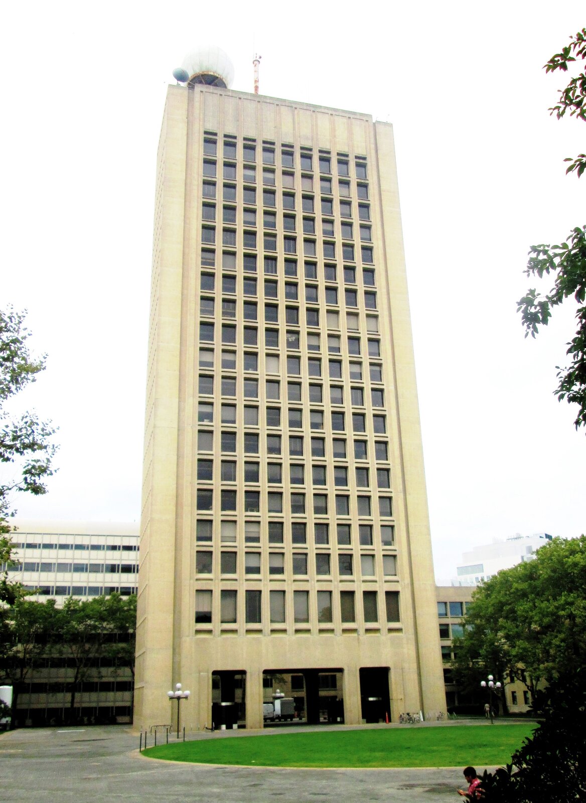
Three years later, in 2011, Daniel Rothman (MIT geophysicist, joined MIT 1986) and Kerry Emanuel (joined 1981) co-founded the Lorenz Center in the MIT School of Science, with the backing of then-Dean Marc Kastner. The center occupies the top floor of the Green Building (Building 54) where Lorenz had spent the bulk of his career. Its declared mission, in Rothman’s and Emanuel’s framing, is to be a “scientific oasis… free of financial and political pressures,” a curiosity-driven climate-research environment explicitly modelled on Lorenz’s own scientific style. The founders argued that the field had drifted toward applied and policy work and needed to recover its theoretical core. Naming the centre after Lorenz, who had been emeritus at MIT until his death, was the natural choice: his entire scientific style – working alone or with a single assistant, pursuing fundamental questions on a small computer, ignoring institutional politics – embodied the curiosity-driven mode the centre intended to encourage. As of 2026 the centre is co-directed by Rothman and Raffaele Ferrari, an Italian ocean dynamicist at MIT EAPS. The centre runs the John Carlson Lectures (an annual public lecture by leading climate scientists), the Lorenz-Houghton Postdoctoral Fellowship, and a visiting scholar programme.
In February 2018, MIT EAPS hosted a Chaos and Climate symposium to mark the joint centennials of Lorenz and Charney (both born 1917). The keynote was given by Ernest Moniz; the panel included Brian Hoskins, Inez Fung, Emanuel, Allison Wing, and John Bush; it was moderated by Robert van der Hilst. Emanuel’s symposium summary line – “history may well record that Ed Lorenz had hammered the last nail into the coffin of Laplace’s daemon” – has stuck. David Randall’s symposium line on Charney – “being in the room with Charney was like being in the room with a tiger, a very friendly tiger” – captures the temperamental contrast at the heart of the MIT department’s twenty-five-year Lorenz-Charney era. Charney the tiger, Lorenz the coyote: complementary, not antagonistic.
The series-wide significance is easier to state than to fully unpack. Lorenz’s 1963 paper transformed pure mathematics, then in turn theoretical physics, then in turn the popular imagination, in roughly twenty-five-year stages. His 1969 paper transformed operational meteorology in roughly twenty-three years (1969 to 1992). His 1995 Lorenz 96 model transformed ensemble data-assimilation research in roughly five years (the late-1990s adoption was almost immediate). By 2026 chaos is the operational substrate of every ensemble forecast made at every centre in the world. The European Centre for Medium-Range Weather Forecasts, Cray-1A serial number nine and forty subsequent generations of supercomputer behind it, runs an ensemble of 50 perturbed members daily out to fifteen days. The American National Centers for Environmental Prediction, Suitland and then College Park, runs the Global Ensemble Forecast System with 31 members. The UK Met Office, Météo-France, the Japan Meteorological Agency, the China Meteorological Administration, the Canadian Meteorological Centre, the Bureau of Meteorology in Melbourne – every one of them runs an operational ensemble derived in some direct or indirect way from Palmer-Molteni-Buizza singular vectors or Toth-Kalnay bred vectors, both grounded in Lorenz 1969.
Whether the modern AI weather models (GraphCast, Pangu-Weather, FourCastNet, FuXi, and their successors) break Lorenz’s predictability barrier is a much-debated question that has been examined elsewhere in this series. The short answer is no: those models are emulating a deterministic forward operator on the same atmosphere, and their useful skill horizon is the same 10-14 day window. What they do better than the conventional models is exploit observational analogs more efficiently and reduce systematic model error; the predictability barrier itself, the upscale-cascade-of-small-errors barrier identified by Lorenz in 1969, has not moved.
There is one more thing to say. The chaos result was, by every account, the kind of discovery that gets called serendipitous. James Gleick put it like this: “Lorenz never was the type to shout Eureka. Serendipity merely led him to a place he had been all along.” A reader-friendly reading of this is that the place Lorenz had been all along was the place where the dynamical equations of the atmosphere meet the actual limited precision of any real device that integrates them. He had been at that intersection since 1942, when his MIT cadet instructors had failed to tell him how to use the dynamical equations to make weather forecasts. He had been at it since 1958, when his Royal McBee LGP-30 arrived and gave him a desktop machine on which the dynamical equations met sixty multiplications per second and six-decimal-place drum memory. He had been at it for two years already in 1961, with Margaret Hamilton’s binary edits on paper tape, when Ellen Fetter came onto the project and the office sweepstake on what the model would do next was running every Monday. When the printout came off the drum slightly different from the day before, with the two trajectories diverging across a few weeks of simulated time from initial conditions that differed in the fourth decimal place, he saw what nobody before him had seen because he was looking at exactly the right place and had been for twenty years.
The right place, for him, turned out to be two decimal places at MIT: the gap between what the Flexowriter printed, three digits, and what the drum memory stored, six. The gap that to any other observer would have looked like a rounding annoyance turned out, in a sufficiently nonlinear deterministic system, to be the gap between coherent forecast and total ignorance. He saw it, became “rather excited,” and spent the next forty-seven years working out what it meant.
He is buried in Cambridge. His personal records and papers are in the MIT Institute Archives. His name is on a centre on the top floor of the Green Building. His 1963 attractor is on physics-textbook covers worldwide. His 1969 horizon is the working ceiling of operational weather forecasting. His 1995 Lorenz 96 is in every introductory data-assimilation course. His birthday, the 23rd of May 1917, is now the date of the annual John Carlson Lecture at MIT.
The man himself was, in his quietest moments at his Cambridge dining-room table after Jane’s death, working through the proofs of the Hénon-map paper that would appear posthumously in Physica D. He had stopped chess by then, but he kept the jigsaw collection. The White Mountains were a fifteen-minute drive from Lexington. He had been to Waterville Valley in every decade of his life, beginning with his parents’ courtship in 1916, eight months before he was born. He had imitated the coyotes in the desert. He had answered when they answered back.
Footnotes
Sources
Primary autobiographical
- Lorenz, E. N., 1991: A scientist by choice. Kyoto Prize Commemorative Lecture, Inamori Foundation.
- Lorenz, E. N., 1993: The Essence of Chaos. University of Washington Press. The 1972 AAAS talk is reprinted as Appendix 1.
- WMO, 1996: The Bulletin interviews Professor Edward N. Lorenz. WMO Bull. 45, 111-120.
- Lorenz, E. N., 2014 (interviewed November 2007): Revisiting the limits of predictability and their implications. Bull. Amer. Meteor. Soc. 95, 681-687.
Lorenz’s key scientific papers
- Lorenz, E. N., 1955: Available potential energy and the maintenance of the general circulation. Tellus 7, 157-167.
- Lorenz, E. N., 1963: Deterministic nonperiodic flow. J. Atmos. Sci. 20, 130-141.
- Lorenz, E. N., 1963: The mechanics of vacillation. J. Atmos. Sci. 20, 448-464.
- Lorenz, E. N., 1967: The nature and theory of the general circulation of the atmosphere. WMO Publication No. 218.
- Lorenz, E. N., 1969: The predictability of a flow which possesses many scales of motion. Tellus 21, 289-307.
- Lorenz, E. N., 1972: Predictability: Does the flap of a butterfly’s wings in Brazil set off a tornado in Texas? AAAS 139th meeting, Washington DC, 29 December 1972. Title coined by Philip Merilees. Reprinted in The Essence of Chaos, 1993.
- Lorenz, E. N., 1982: Atmospheric predictability experiments with a large numerical model. Tellus 34, 505-513.
- Lorenz, E. N., 1986: On the existence of a slow manifold. J. Atmos. Sci. 43, 1547-1557.
- Lorenz, E. N., 1995: Predictability: A problem partly solved. ECMWF Seminar on Predictability, Reading.
Biographies and obituaries
- Emanuel, K., 2011: Edward Norton Lorenz, 1917-2008. Biographical Memoirs of the National Academy of Sciences, Washington DC.
- Palmer, T. N., 2009: Edward Norton Lorenz. 23 May 1917 - 16 April 2008. Biographical Memoirs of Fellows of the Royal Society 55, 139-155. The full text was unavailable for this post due to a paywall on royalsocietypublishing.org; cited via Emanuel.
- MIT News, 16 April 2008: Edward Lorenz, father of chaos theory and butterfly effect, dies at 90.
- The Tech (MIT student paper), 18 April 2008: Edward N. Lorenz ScD ‘48.
- Physics Today online obituary, April 2008.
- The Times of London obituary, April 2008; republished on the MacTutor History of Mathematics archive at St Andrews.
- Britannica biography, Edward Lorenz.
Secondary scientific
- Saltzman, B., 1962: Finite amplitude free convection as an initial value problem - I. J. Atmos. Sci. 19, 329-342.
- Ruelle, D., and Takens, F., 1971: On the nature of turbulence. Commun. Math. Phys. 20, 167-192.
- Li, T.-Y., and Yorke, J. A., 1975: Period three implies chaos. Amer. Math. Monthly 82, 985-992.
- Gleick, J., 1987: Chaos: Making a New Science. Viking. Chapter 1, “The Butterfly Effect.”
- Motter, A. E., and Campbell, D. K., 2013: Chaos at fifty. Physics Today 66(5), 27-33.
- Sokoler, J., Yoder, S., and Gabai, J., 2019: The hidden heroines of chaos. Quanta Magazine, 20 May 2019.
- Zhang, F., Sun, Y. Q., Magnusson, L., Buizza, R., Lin, S.-J., Chen, J.-H., and Emanuel, K., 2019: What is the predictability limit of midlatitude weather? J. Atmos. Sci. 76, 1077-1091.
- Shen, B.-W., and Pielke, R. A. Sr., and others, 2024: Lorenz’s view on the predictability limit of the atmosphere. MDPI Encyclopedia 3, 887-905.
The 1992 ensemble launches
- Toth, Z., and Kalnay, E., 1993: Ensemble forecasting at NMC: The generation of perturbations. Bull. Amer. Meteor. Soc. 74, 2317-2330.
- Molteni, F., Buizza, R., Palmer, T. N., and Petroliagis, T., 1996: The ECMWF Ensemble Prediction System: Methodology and validation. Quart. J. Roy. Meteor. Soc. 122, 73-119.
- Palmer, T. N., 2019: The ECMWF ensemble prediction system: Looking back (more than) 25 years and projecting forward 25 years. Quart. J. Roy. Meteor. Soc. 145 (S1), 12-24.
LGP-30 hardware
- Wikipedia, LGP-30, accessed 2026.
- masswerk.at, 2019: LGP-30: A drum computer of significance.
- ed-thelen.org, LGP-30 page (manuals and specifications).
Institutional MIT history
- MIT EAPS, “About Us / History” web pages.
- MIT News, 2011: Wind, war and weathermen.
- MIT News, 2018: Chaos and climate: Celebrating two pioneers of modern meteorology.
- Lorenz Center, MIT, www.lorenz.mit.edu.
- Phillips, N. A., 1995: Jule Gregory Charney. Biographical Memoirs NAS 66, 80-113.
-
Emanuel records the quote on page 16 of the 2011 NAS Biographical Memoir, attributing it to Lorenz’s own retelling of the discovery in interviews and in The Essence of Chaos. The complete quote in context is: “I started the computer, and went to lunch. When I came back about an hour later, the computer had simulated about two months of weather. The numbers being printed out were nothing like the old ones. I immediately suspected a weak vacuum tube or some other computer trouble, which was not uncommon, but before calling for service I decided to see just where the mistake had occurred, knowing that this could speed up the servicing process. Instead of a sudden break, I found that the new values at first repeated the old ones, but soon afterward differed by one and then several units in the last decimal place, and then began to differ in the next to the last place and then in the place before that. In fact, the differences more or less steadily doubled in size every four days or so, until all resemblance with the original output disappeared somewhere in the second month. This was enough to tell me what had happened: the numbers that I had typed in were not the exact original numbers, but were the rounded-off values that had appeared in the original printout. The initial round-off errors were the culprits; they were steadily amplifying until they dominated the solution. In today’s terminology, there was chaos. At this point, I became rather excited.” ↩
-
The Tech (MIT student paper), “Edward N. Lorenz ScD ‘48,” 18 April 2008. The Emanuel quote was given specifically to The Tech; it does not appear in the more formal NAS memoir. It is the only “coyote” reference in the obituary literature and is exactly the kind of personal-recollection detail that gets stripped out of the formal scientific memoirs. ↩
-
The Charney “soul of an artist” quote is preserved in the MIT meteorology oral tradition and is cited by Emanuel in the NAS memoir, attributing it to Charney’s verbal characterisation of Lorenz at MIT department gatherings. I have not located it in a published Charney source. ↩
-
The Physics Today obituary, by the editorial staff (April 2008 online), used this construction explicitly as a hypothetical Lorenz response to the tributes. The line was widely re-quoted in subsequent obituaries and has become a representative summary of his self-effacement. ↩
-
Emanuel NAS memoir, pages 1-3, draws extensively on Lorenz’s own 1991 Kyoto autobiographical lecture for the childhood details. The MIT two-mile-run record, the jigsaw puzzles, the Waterville Valley summers, and the eight-year-old viewing of the 24 January 1925 total solar eclipse are all from this source. The eclipse path of totality crossed Connecticut and southern New England that day; the shadow-bands-on-snow detail is unusual and is the kind of physical observation that probably did stay with him. ↩
-
From Lorenz’s 1991 Kyoto Prize Commemorative Lecture, “A Scientist by Choice,” as quoted in Emanuel NAS memoir page 4. The full sentence is: “It soon became evident that we were studying to be meteorologists. The distinction is one that I was slow to appreciate.” ↩
-
The original title was “Deterministic Turbulence.” The JAS editor required the change to “Deterministic Nonperiodic Flow.” The provenance is given in the Physics Today “Chaos at Fifty” essay (Motter and Campbell 2013). ↩
-
The LGP-30 specifications – 113 vacuum tubes, 1450 diodes, 4096 31-bit words, 3700 rpm drum, approximately 60 multiplications per second, weight roughly 800 pounds, price approximately 47000 1956 dollars – are documented in the Wikipedia LGP-30 article, the masswerk.at “LGP-30: A Drum Computer of Significance” (2019), and the ed-thelen.org LGP-30 page. Gleick’s Chaos (1987) is the canonical popular source for the 60 multiplications per second figure. The looser “about 1 multiplication per second” that appears in some popular sources is wrong by roughly two orders of magnitude. ↩
-
Lorenz, “A Scientist by Choice,” 1991 Kyoto Prize Commemorative Lecture, quoted in Emanuel NAS memoir. ↩