In 1963 the Leningrad publishing house Gidrometeoizdat brought out a 286-page Russian monograph by a 48-year-old meteorologist at the Voeikov Main Geophysical Observatory. The title was “Объективный анализ метеорологических полей” – Obyektivny analiz meteorologicheskikh polei, Objective Analysis of Meteorological Fields. The author was Lev Semyonovich Gandin.1 Two years later, in Jerusalem, the Israel Program for Scientific Translations brought out an English version: Objective Analysis of Meteorological Fields, vi + 242 pages, 53 figures, 28 tables, with the Stanford catalogue note “Available through U.S. Department of Commerce, Clearinghouse for Federal Scientific and Technical Information, Springfield, Virginia.”2 The publisher had taken a Soviet monograph in Russian, translated it into English, and distributed it through the bureaucratic channel that the United States government maintained for the import of Soviet-bloc scientific literature. The Cold War scientific transmission worked in both directions, but it worked more efficiently in the Soviet-to-Western direction than in the reverse. The book that crossed the Iron Curtain in 1965 was one of the more consequential examples of the period.
Twenty-eight years after the Russian original was published, its author – who had spent the previous four decades working entirely within the Soviet meteorological system, who had been a young researcher during the Siege of Leningrad in his late twenties, who had built his career at a single Leningrad observatory, who had emerged into international view only at the very end of his working life – walked into the National Meteorological Center at Suitland, Maryland. At NMC his statistical methods had been the operational reality since 1979. The first generation of analysts who had implemented them in Washington – John Bergman, Stephen Lord, Joseph Sela, and the supporting NMC software team under Frederick Shuman’s directorship – had read the 1965 English translation rather than the 1963 Russian original; almost none of them had Russian. The man in whose 1963 monograph the algorithms had first been written down arrived as a senior émigré scientist, age 76, with John Derber and David Parrish working a few doors away on what would become, on 25 June 1991, the world’s first operational three-dimensional variational analysis system.3 The Soviet-American closure of the OI loop that had been opened in Leningrad in 1963 was complete.

This post is the story of the 1963 monograph, of the man who wrote it, and of the four-cultural intellectual relay that turned its central idea – objective analysis as a minimum-variance linear estimation problem – into the operational data assimilation systems of every major weather centre on Earth.4 The relay is the story’s spine: Bergthorsson and Doos in Scandinavia in 1955, Cressman at the United States Joint Numerical Weather Prediction Unit in 1959, Gandin at Leningrad in 1963, Lorenc at the European Centre for Medium-Range Weather Forecasts in 1981, Parrish and Derber at NMC in 1991, ECMWF following NMC into the variational era in 1996 and 1997, and the Canadian Meteorological Centre putting the first operational Ensemble Kalman Filter into routine production on 12 January 2005. The path runs from Reykjavik and Stockholm through Washington and Leningrad to Reading and back, with each centre adding a piece of the framework that the next centre would extend. It takes seventy years to complete. The names along the way matter, but the idea that the four cultures all converge on is the same idea: that the analysis of a weather field is a statistical inference problem in which the answer is the linear combination of background and observations that minimises an expected squared error. Everything since 1963 has been the elaboration of that formulation.
Where this post fits
The earlier post in this series on Norman Phillips at NMC covered the man who was Principal Scientist of NMC’s Development Division through the entire OI deployment, from 1974 to the mid-1980s.5 Phillips’s tenure at the World Weather Building at Suitland is the institutional bridge that this post sits on. The OI scheme that John Bergman implemented in 1979 was the first major NMC analysis change of Phillips’s time as Principal Scientist; the transition to 3D-Var on 25 June 1991 was the last major analysis change before he had fully retired. Phillips read the 1965 IPST translation of Gandin’s monograph at MIT in the 1960s, brought the framework with him to NMC in 1974, and oversaw the operational engineering that turned the Russian-Leningrad theory into the American-Suitland practice. The same is true at the other geographical pole of the post: at ECMWF in Reading, Anthony Hollingsworth as Head of Research from 1990 led the trajectory from the Lorenc 1981 OI through the empirical Hollingsworth-Lonnberg structure functions of 1986 to the 3D-Var and 4D-Var implementations of the 1990s.
The post on Frederick Shuman’s seventeen years at Suitland covered the operational shop in which NMC’s OI lived through its first decade.6 The Bergman OI implementation of 1979 was a Shuman-era artefact: Shuman authorised the procurement of the Cyber 205 (delivered August 1983, after Shuman retired in January 1981 but planned during his last year), authorised the Global Spectral Model development that would feed observations into the OI, and presided over the eight-year run of OI as the operational analysis at NMC from 1979 to 1991. The story of Shuman’s NMC and the story of Gandin’s Leningrad converge at the moment in 1991 when the spectral statistical interpolation system superseded both – but built on both.
The post on Edward Lorenz covered the man whose 1969 Tellus paper became the theoretical foundation of every operational ensemble system on Earth.7 The connection back to the present post is direct. The Hollingsworth-Lonnberg 1986 Tellus paper that gave operational OI its empirical structure functions, and which the present post will return to in its sixth section, was a direct outgrowth of the predictability framework Lorenz had built up over the 1960s and 1970s. The deterministic-forecast horizon Lorenz had pinned down in 1969 was the same horizon that the data assimilation community was, in 1986, trying to push out by improving the analysis. The two trajectories – predictability theory and data assimilation theory – are the two halves of the same conversation about how to extract maximum signal from a noisy, partially observed, chaotic system.
The post on Bracknell’s Cyber 205 covered the Met Office in the 1980s, where Andrew Lorenc – before moving to ECMWF in the late 1970s, then back to the Met Office in 1980 – led the development of the global multivariate OI scheme.8 The 1981 Lorenc MWR paper is the canonical Western adaptation of Gandin’s framework; it is the next link in the chain after Gandin’s 1963 monograph and before Parrish and Derber’s 1991 SSI. It is the moment at which the Soviet theory became the British operational practice and, through the parallel ECMWF adoption, the European operational practice.
1. Before Gandin: the Scandinavian and American roots
The history of objective analysis in operational meteorology starts not in Leningrad but in Stockholm. In 1954 two young Scandinavian meteorologists, Pall Bergthorsson (Icelandic) and Bo Doos (Swedish), working at the Internationella Meteorologiska Institutet in Stockholm under Carl-Gustaf Rossby’s leadership, produced a method for converting the hand-drawn analyses that synoptic forecasters had been making for half a century into the gridded fields that the new numerical models – the ENIAC integration of March 1950 was only four years old – required as input.9 The Bergthorsson-Doos method was published in 1955 in Tellus 7, the journal Rossby had founded in 1949 with explicit purpose of giving Scandinavian and continental European meteorology an international outlet: “Numerical weather map analysis.”10
The Bergthorsson-Doos algorithm was elementary. At each grid point of the analysis, the method took as background the climatological mean for the time of year and the location. It then corrected the background at the grid point by a distance-weighted average of the differences between the radiosonde observations around the point and the background interpolated to the observation locations. The weights were a function of the distance from the grid point to the observation. As you moved further from any observation, your analysis fell back toward the climatology; as you moved into a dense observation network, your analysis tracked the observations. The method was, in modern language, a successive-corrections analysis with a climatological background and a distance-only weighting function. It had no statistical justification, no derivation from a minimum-variance principle, no multivariate coupling between mass and wind. It worked because the climatological background was a reasonable first guess and because the radiosonde network was dense enough over Scandinavia and Europe to constrain the analysis.
The Bergthorsson-Doos method is the Scandinavian fourth-cultural anchor of the lineage this post tracks. It is the first paper in the open meteorological literature to express the objective analysis problem in terms a computer can carry out without subjective input from a human analyst. Everything that came afterward – Cressman in 1959, Gandin in 1963, Lorenc in 1981 – elaborated on the same basic structure: a background field plus a weighted correction from the observations. The disagreement was about the weights, the background, and the statistical interpretation of both. Bergthorsson and Doos had picked the weights by intuition and the background by climatology; their successors would pick both by minimum-variance arguments.
The next link in the chain came at the Joint Numerical Weather Prediction Unit in Suitland, Maryland, four years after Bergthorsson-Doos. The Unit had been founded on 1 July 1954, jointly by the United States Weather Bureau, the Air Weather Service, and the Naval Weather Service, to put numerical weather prediction onto an operational footing in the United States.11 Its first operational forecast had been on 6 May 1955. In 1958 the Unit ran on an IBM 704 with a hemispheric grid of 1977 points at one and a half levels in the vertical; the analysis problem – converting the daily radiosonde, surface, and ship observations into gridded values that the model could consume – was being done by George Cressman, the Unit’s director from 1957 onward.12
Cressman’s 1959 paper “An Operational Objective Analysis System,” in Monthly Weather Review 87, 367-374, became the canonical reference for the successive-corrections family of methods.13 At each grid point $i$, Cressman wrote the analysis $x_a(i)$ as the background $x_b(i)$ plus a weighted correction:
\[x_a(i) = x_b(i) + \frac{\sum_j w(i,j) [y(j) - x_b(j)]}{\sum_j w(i,j)}\]where $y(j)$ are the observations indexed by $j$, $x_b(j)$ is the background interpolated to observation location $j$, and the weight $w(i,j)$ falls smoothly from one at zero distance to zero at a user-chosen “influence radius” $R$:
\[w(i,j) = \max\left(0, \frac{R^2 - d_{ij}^2}{R^2 + d_{ij}^2}\right)\]with $d_{ij}$ the distance between grid point $i$ and observation $j$. A second pass through the algorithm with a reduced influence radius $R$ corrected the analysis for smaller-scale features; some implementations iterated through three or four passes with progressively smaller radii. The background was now the previous-cycle forecast rather than climatology – a substantive improvement over Bergthorsson-Doos – but the weighting function was still chosen by intuition and was still purely a function of distance. The method was univariate: each variable (height, temperature, wind component) was analysed independently of the others, with no coupling between mass and wind.
Cressman’s scheme ran in operations at the JNWPU, and at its successor the National Meteorological Center after the 1958 reorganisation, for twenty years. It was the workhorse of American operational analysis from 1959 to 1979.14 It ran on an IBM 7090, then on a 360/30, then on a 360/195 from 1968, and finally for a brief period on the Cyber 205 from 1983 while the OI transition was being completed. Through the 1960s and into the 1970s, every major NWP centre in the world ran some variant of successive corrections as its operational analysis: NMC, ECMWF predecessors, JMA, the Met Office, the Canadian Meteorological Centre, the Air Force Global Weather Central, FNOC, GFDL’s research analyses for climate simulations. The scheme was simple, fast, and known to work as long as the observation network was dense enough and the analysis cycle was short enough.
It started to fail in the 1970s. The observation mix diversified. TIROS-N in 1978, NOAA-6 in 1979, and NOAA-7 in 1981 were operational sun-synchronous satellites carrying the TIROS Operational Vertical Sounder (TOVS) – the High Resolution Infrared Radiation Sounder (HIRS), the Microwave Sounding Unit (MSU), and the Stratospheric Sounding Unit (SSU) – which delivered temperature retrievals at thousands of points per day over the data-sparse oceans and the southern hemisphere. Aircraft observations through the AIREP and ACARS reporting systems delivered wind and temperature reports at flight level. Drifting buoys and moored buoys in the Drake Passage, the Southern Ocean, and the equatorial Pacific delivered surface pressure and sea-surface temperature. Each new observation type had its own error variance, its own spatial correlation, its own vertical-coverage characteristics. The Cressman weighting function, which knew nothing about the relative accuracy of background and observation and nothing about cross-variable correlations, could not represent any of this.
The geostrophic coupling between mass and wind was the second failure of Cressman. On synoptic scales the wind field is approximately the geostrophic wind, determined by the horizontal gradient of the geopotential height; a height observation therefore carries information about the wind, and a wind observation carries information about the height. Cressman’s univariate scheme could not exploit this coupling. The analysis of the height field used height observations, the analysis of the wind used wind observations, and the two fields could end up inconsistent with each other in ways that the dynamical model then had to spin down through initialisation – an unwelcome additional step that introduced its own model-dependent errors.
What the operational community needed in 1975 – when the Bergman team at NMC was beginning the work that would put OI into operations – was a statistical framework that could (a) weight observations by their relative accuracy, (b) couple mass and wind through their geostrophic correlation, and (c) extrapolate the information from each observation according to the empirically determined correlation structure of the atmosphere rather than according to a distance-only weighting. The framework already existed. It had been published in Leningrad in 1963 and translated in Jerusalem in 1965. It just needed to be found by people who could read it and operationalised by people who could code it.
2. Gandin at Leningrad
Lev Semyonovich Gandin was born in 1915 – the year of the third year of the First World War, two years before the Russian Revolution, in the city that would, three centuries earlier, have been Saint Petersburg and that within a decade of his birth would be renamed Leningrad after Lenin’s death in January 1924.15 He died in 1997 in the Washington, D.C. area, age 82, after six years as a UCAR Scientist at the National Meteorological Center.16 His life therefore spanned the whole twentieth-century history of Russian meteorology: the imperial Main Physical Observatory that had hosted Amundsen in 1907 was still the same institution, in the same building, when Gandin began working there in his early thirties; the post-Soviet Russian Federation Roshydromet was three decades old when he emigrated and six years old at his death.
The birth year matters for the framing. At the publication of the 1963 monograph he was 48 years old.17 He was not a young man making his name with a doctoral thesis; he was a senior Soviet meteorologist with two decades of working experience, synthesising a programme of research that had run through the Trudy GGO – the proceedings of the Voeikov Main Geophysical Observatory – since the late 1940s. The monograph was the gathering-in of a career’s first half, not its opening. By 1988, when the MWR paper on Complex Quality Control appeared with what the secondary literature suggests was an NMC affiliation, Gandin was 73; by his arrival at NMC in 1991 he was 76. He was, in every sense, a senior émigré scientist – not the young Soviet defector or post-Soviet brain-drain trainee whom the late-1990s American science press chronicled, but a working scientist at the end of a long career, joining an American operational shop that had already been running his methods for twelve years before he set foot in it.
The factual record of Gandin’s early life is thin in English-language sources. He worked at the Main Geophysical Observatory from sometime in the late 1940s – the IMSC citation given by his longtime Soviet colleague G. V. Gruza at the 1992 Toronto meeting fixes the institutional link: “All scientific activities of Lev Gandin up to 1981 were connected with the Main Geophysical Observatory in Leningrad, now St. Petersburg.”18 His first research was on “the physics of the surface air layer and vertical turbulent exchange,” boundary-layer micrometeorology of the Soviet style that Andrey Monin and Alexander Obukhov were then making canonical with the 1954 Monin-Obukhov similarity theory. Gandin worked alongside and under the long shadow of Mikhail Budyko (1920-2001), the great Soviet climatologist who from 1954 to 1972 was the head of MGO.19
What we know about Gandin himself as a person comes principally from one source: Gruza’s 1992 citation, reproduced in International Journal of Climatology by Allan Murphy and Francis Zwiers in 1993. The citation calls Gandin “very young, very clever, and a very cheerful fellow” – this is the recollection of the 1950s, when Gandin was in his late thirties – known for “endless jokes and sharp remarks.” He was “an excellent lecturer” and authored “several very good handbooks and monographs for students, graduates, and postgraduates.” Outside meteorology he was a strong ping-pong player, a leading chess player, a bridge player, and “plays the piano beautifully.”20 The cultivated polymathic profile is the standard one for senior Soviet academic scientists of the 1950s and 1960s generation – the same generation that produced Kolmogorov’s mathematical school in Moscow, Yaglom’s probability-and-turbulence work, and the broader Soviet tradition of mathematical rigour applied to physical problems. Gandin fitted that tradition closely.

The Siege of Leningrad ran from 8 September 1941 to 27 January 1944 – twenty-eight months of German encirclement that killed approximately one million civilians from starvation, hypothermia, and bombardment. Gandin was 26 at the start of the siege and 29 at its end. He was a working meteorologist at the Main Geophysical Observatory through it. Whether he was on the staff of the observatory itself, evacuated with the institution’s relocation to safer cities further east, or stationed at one of the Leningrad-Front military observation posts that fed weather data to the Soviet bomber and artillery commands – the open record I have access to does not say. The biographical entry in the Lev_Gandin.md research note for this post is explicit: “FACT NOT VERIFIED” on the siege period. What is documented is that his research career, by Gruza’s account, “began just after the Second World War” – meaning that the wartime work, whatever it was, did not contribute substantively to the postwar publication record. The siege is in his biography as a survived experience, not as a publication-producing one. His scientific reputation begins around 1947 or 1948 with the boundary-layer turbulence papers.
By the late 1950s Gandin had moved his research from boundary-layer turbulence to the statistical structure of meteorological fields. The shift fits the institutional logic of MGO: Budyko’s leadership from 1954 was pushing the observatory toward large-scale climatological synthesis, and the radiosonde network that the Soviet hydrometeorological service had been building since the 1930s was now dense enough – over European Russia, the Trans-Baikal, the Far East, the Soviet Arctic – to allow the empirical autocorrelation structure of geopotential height to be estimated. The technical question Gandin set himself was the one this whole post is about: how do you take a set of irregularly-spaced radiosonde observations and produce a gridded analysis that, in some statistically defensible sense, minimises an expected error?
The mathematical tradition Gandin worked in was, by the standards of mid-1950s Western applied mathematics, very strong. Andrey Kolmogorov had founded modern probability theory in the 1930s; his 1941 papers on the Kolmogorov spectrum of three-dimensional isotropic turbulence had given Soviet fluid dynamicists the conceptual scaffold to think in terms of statistical structure functions. Norbert Wiener’s 1949 Extrapolation, Interpolation, and Smoothing of Stationary Time Series had introduced linear least-mean-square prediction and filtering for one-dimensional stationary processes. Aleksandr Khinchin had developed the Wiener-Khinchin theorem connecting power spectra and autocorrelation functions. Akiva Yaglom, working in Moscow at the Institute of Atmospheric Physics from the 1950s, had carried the theory into the two- and three-dimensional vector random-field setting that meteorology needed. Gandin’s contribution – the part that made him a name internationally rather than just nationally – was to translate this body of mathematical theory into a sequence of algorithmic recipes that an operational meteorologist could actually execute on the computers of the period.21
3. The 1963 monograph
What Gandin published in 1963 is, in modern language, the Best Linear Unbiased Estimator (BLUE) framework applied to objective analysis of meteorological fields. The framework is now standard, and runs as follows. Suppose you have a true state vector $\mathbf{x}^t$ of dimension $n$ – the values of the geopotential height, temperature, and wind at every grid point of an analysis domain. You have a background state $\mathbf{x}^b$ of the same dimension, the previous cycle’s forecast interpolated to the analysis grid, with error $\mathbf{x}^b - \mathbf{x}^t$ whose covariance matrix is $\mathbf{B}$ of size $n \times n$. You have an observation vector $\mathbf{y}$ of dimension $p$, with observation operator $\mathbf{H}$ mapping the model state to the observation space (the simplest case is linear interpolation from grid points to radiosonde locations) and observation error covariance $\mathbf{R}$ of size $p \times p$. Then the analysis state $\mathbf{x}^a$ that minimises the expected analysis error variance is
\[\mathbf{x}^a = \mathbf{x}^b + \mathbf{K} (\mathbf{y} - \mathbf{H} \mathbf{x}^b)\]with the Kalman gain matrix
\[\mathbf{K} = \mathbf{B} \mathbf{H}^T (\mathbf{H} \mathbf{B} \mathbf{H}^T + \mathbf{R})^{-1}\]The analysis error covariance is $\mathbf{A} = (\mathbf{I} - \mathbf{K}\mathbf{H}) \mathbf{B}$. If the background and observation errors are Gaussian, the BLUE is also the maximum-likelihood estimate; the same answer comes out of a minimum-variance derivation and out of a Bayesian one.22 The formulation is, in 2026 terms, second-year graduate-school material in any data assimilation course.
The plain-language version, before any formula: the analysis is a weighted average. You take the background and you take the observations. The weights depend on how much you trust each. If you trust the background more (because the model has been performing well), the analysis stays close to the background. If you trust the observations more (because they are recent radiosondes from a dense network), the analysis pulls toward the observations. The clever part is what “trust” means quantitatively: it means the inverse covariance matrices $\mathbf{B}^{-1}$ and $\mathbf{R}^{-1}$, which capture not just how big the errors are but also how they are correlated between different points. If two nearby grid points have correlated background errors (because the model gets a whole pressure system wrong as a unit), then an observation that corrects one of them carries information about the other. If two observations have correlated errors (because they come from the same satellite pass), then their combined information is less than the sum of the parts. The whole game is the bookkeeping of these correlations.
This is the framework Gandin wrote down in 1963.23 His central technical innovation, beyond stating the framework in clean meteorological notation, was the autocorrelation-function approach to the background error covariance $\mathbf{B}$. The full $n \times n$ background error covariance matrix has approximately $n^2/2 \approx 5 \times 10^{13}$ independent entries for a modern operational model with $n \sim 10^7$, which cannot be specified or stored. Gandin’s recipe was: assume horizontal homogeneity and isotropy of the background errors. That is, assume that the covariance of the background error in geopotential height at two points depends only on the distance between them, not on the absolute position of either point and not on the orientation of the line joining them. Under that assumption, $\mathbf{B}$ reduces to a one-dimensional function of separation distance $r$, the autocorrelation function $\mu(r)$, which can be estimated empirically from a few hundred archived radiosonde forecast-error pairs.
Gandin tabulated empirical $\mu(r)$ functions from Soviet radiosonde data. The function he proposed for geopotential height was approximately exponential or Gaussian, with an e-folding scale of several hundred kilometres – the “Gandin function” of later Western literature. The exact functional form varied across the monograph and across the implementations that followed, but the conceptual move – replace the impossible $n^2$ matrix with a one-dimensional empirical function – was universal.24 In the vertical, Gandin assumed separability: the full three-dimensional autocorrelation factored as a product of a horizontal function and a vertical function, with the vertical function fit empirically from radiosonde data at standard pressure levels.
The Gandin construction also handled the multivariate coupling between mass and wind. Under the assumption that the background errors satisfied the geostrophic balance to a good approximation – which they do on synoptic and larger scales – the cross-covariance between height errors at one point and wind errors at another could be derived analytically from $\mu(r)$ by differentiation. A single observation of geopotential height, fed through $\mathbf{B}\mathbf{H}^T$, produces a circularly-symmetric height increment surrounded by a ring of rotational wind increment – the classic structure function picture that every NWP textbook reproduces. A single observation of wind, conversely, produces an increment in the height field corresponding to a small low-pressure or high-pressure feature in the right place to make the wind geostrophically consistent. The multivariate coupling fell out of the geostrophic assumption and the autocorrelation function; it did not need to be specified separately.
The third technical move in the 1963 monograph was the local data selection approximation. The full BLUE computation requires inverting a $p \times p$ matrix $(\mathbf{H}\mathbf{B}\mathbf{H}^T + \mathbf{R})$ at cost $O(p^3)$, where $p \sim 10^5$ is the number of observations per analysis. This was infeasible on the computers of the 1960s and of the 1970s and – borderline – of the 1980s. Gandin’s approximation: for each grid point of the analysis, select only the $p_i \sim 50$ to $100$ observations nearest to that grid point, and form the BLUE using only those. The local matrix inverse is $O(p_i^3) \sim 10^6$ operations, which is small. The analysis at each grid point is independently locally optimal, but globally the analysis is a patchwork of local solutions with arbitrary selection radii. The cost of the approximation is twofold: visible “tile-boundary” artefacts where the selected observation set changes from one grid point to the next, and the loss of strict global optimality. The benefit – the only reason OI was operationally tractable in 1979 – was that the computational cost dropped from $O(p^3)$ to $O(n \cdot p_i^3)$, which is small enough to run on the IBM 360/195 of NMC’s 1979 hardware.25
These three moves – the autocorrelation-function approach to $\mathbf{B}$, the geostrophic multivariate coupling, and the local data selection – are the technical heart of what became known in the West as Optimal Interpolation, or OI. The 1963 Russian monograph contained all three. The 1965 English translation transmitted them to the West. Operational implementations followed within fifteen years.
4. The 1965 translation
The Israel Program for Scientific Translations (IPST) was a Jerusalem-based scientific publisher founded in 1959 specifically to translate Soviet and Eastern European scientific monographs into English for distribution in the West. Its main funding source was contracts with United States federal agencies: the National Science Foundation, NASA, the Department of Commerce, the Department of Health, Education and Welfare, the Atomic Energy Commission. Through the 1960s and 1970s, IPST produced several hundred translations of Russian scientific monographs across mathematics, physics, chemistry, biology, geology, meteorology, oceanography, and engineering. The programme was one of the larger pieces of Cold War intellectual transmission infrastructure, comparable in scale to the simultaneous Soviet programme of translating Western scientific literature into Russian (which produced, for example, the Russian editions of Wiener’s Cybernetics and of Feynman’s Lectures on Physics).26
The 1965 English edition of Gandin’s monograph – Objective Analysis of Meteorological Fields, translated by R. Hardin, vi + 242 pages, 53 figures, 28 tables, OCLC 25601011 – was produced under the standard IPST template. The Stanford SearchWorks catalogue records the distribution channel: “Available through U.S. Department of Commerce, Clearinghouse for Federal Scientific and Technical Information, Springfield, VA.”27 The Clearinghouse for Federal Scientific and Technical Information (CFSTI) had been established by the Federal Council for Science and Technology in 1964, consolidating earlier federal technical-document distribution programmes; it would in 1970 be renamed the National Technical Information Service (NTIS) under the Department of Commerce. The Gandin translation thus had a specific bureaucratic identity in the United States federal technical-document system: it was a Department of Commerce CFSTI item, available by mail order to American libraries, universities, and government laboratories.
This is the version that the Western data assimilation community read. Andrew Lorenc read it as a graduate student at Imperial College London in the early 1970s, before moving to the Met Office and then to ECMWF.28 Lennart Bengtsson read it at the Swedish Meteorological and Hydrological Institute before moving to ECMWF as its Head of Research and then Director. John Bergman, Stephen Lord, Joseph Sela, and the rest of the NMC analysis-development team read it through the 1970s.29 Peter Lonnberg and Anthony Hollingsworth read it at ECMWF before producing the 1986 Tellus structure-function paper that built on Gandin’s framework. Almost none of them read the 1963 Russian original. The 1965 English translation was, for the Western community, the foundational document.
The Internet Archive scan of the 1965 IPST edition, at archive.org/details/objectiveanalysi0000lsga, is the primary source for the present post.30 The QJRMS review of the translation, by John Sawyer (or, by some attributions, Geoffrey Howard) at the Met Office, appeared in Quarterly Journal of the Royal Meteorological Society Vol. 92, p. 447, in 1966 – the first substantive Western signal that the monograph existed and was worth reading.31 The review was favourable but cautious; it noted that the methods were “more elaborate than is justified by the present density of the observational network” but recognised that they would become increasingly important as the network grew. The review’s prediction – that the methods would become important later – turned out to be correct, but the timescale was longer than Sawyer estimated: fourteen years from the review (1966) to the first operational NMC implementation (1979) to the routine use across all major Western centres by the mid-1980s.
The transmission was slow not because the methods were obscure but because the operational engineering of them required substantial work. The 1963 monograph specified the framework but did not give a turnkey implementation. The autocorrelation function had to be fit to a specific centre’s radiosonde data. The local data selection had to be tuned against the centre’s specific observation density. The vertical structure of $\mathbf{B}$ had to be estimated from the centre’s specific forecast model. The interpolation operator $\mathbf{H}$ had to be coded for the centre’s specific analysis grid. None of this was conceptually difficult, but all of it was time-consuming, and through the late 1960s and early 1970s the operational centres were busy with other things: the transition from baroclinic models to multi-level primitive-equation models, the implementation of spectral transforms, the introduction of satellite data, the rollout of new computers. Objective analysis was not the most urgent problem on most operational shop’s lists. It became urgent in the mid-1970s, when the diversification of the observation network made the limits of Cressman successive corrections obvious, and the operational implementations followed within five years.
5. The 1979 NMC implementation
The Western operational adoption of OI began at the National Meteorological Center in 1979, under John Bergman in the Development Division and with Norman Phillips as the Principal Scientist of the Division. The implementation is documented in Bergman’s 1979 MWR paper “Multivariate analysis of temperatures and winds using optimum interpolation,” Monthly Weather Review 107, 1423-1444, and in its companion paper “The NMC Operational Global Data Assimilation System,” MWR 107, 1445-, by the analysis-team senior author and Bergman as coauthor.32 The work was a direct application of the Gandin framework to the NMC observational data set, the NMC global spectral model background, and the NMC operational computer of the period (an IBM 360/195 with 4 megabytes of memory, sustaining roughly 10 megaflops on the analysis workload, transitioning to the Cyber 205 in 1983).
The system Bergman built was multivariate in height and wind, three-dimensional in the vertical, and used the Gandin local-data-selection approximation with approximately 50 observations per analysis grid point. The autocorrelation function was fit to NMC’s archived radiosonde forecast-error pairs over the previous several years. The vertical correlations were specified separately at standard pressure levels (1000, 850, 700, 500, 400, 300, 250, 200, 150, 100, 70, 50 hPa) with a separability assumption. The observation error covariances were assumed diagonal for radiosondes, with off-diagonal terms for satellite retrievals where the inter-channel error correlations were thought to be significant.33 The analysis ran twice daily, 00 and 12 UTC, with a six-hour assimilation cycle in which the previous six-hour forecast became the background for the next analysis.
The performance gain over the prior Cressman scheme was substantial. Forecast verification scores improved by roughly the equivalent of half a day at the medium range: the 72-hour forecast from the OI analysis was as skilful as the 60-hour forecast from the Cressman analysis had been. The improvement was attributable in roughly equal parts to (a) the multivariate coupling of mass and wind, which gave geostrophically balanced initial conditions that the model could spin up cleanly without long initialisation transients, (b) the use of empirically-determined autocorrelation functions rather than a Cressman influence-radius cone, which extracted more information from each observation, and (c) the proper accounting for observation error variances, which downweighted the noisier satellite retrievals relative to the more accurate radiosondes.
The NMC OI ran in operations from 1979 to 1991. Through that twelve-year operational life, the scheme was incrementally refined: new observation types added (TOVS radiances from 1981, aircraft reports from the late 1970s, drifting buoys from the early 1980s, scatterometer winds from SEASAT briefly and from ERS-1 from 1991), the autocorrelation function tuned, the vertical levels extended, the data-selection radii adjusted. Joseph Sela and the NMC global spectral model team upgraded the underlying forecast model from rhomboidal truncation R30 with twelve vertical levels to R40 with twelve levels in 1980, then to T80 with eighteen levels around 1985, then to T126 in the late 1980s; the OI analysis grid followed the spectral resolution upward.34 Eugenia Kalnay, who became Director of NMC’s Development Division in 1987, oversaw the second half of the OI era and the transition to its successor.
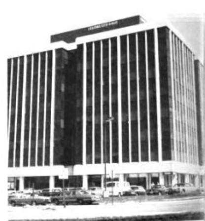
The institutional environment in which OI ran at NMC through the 1980s was the World Weather Building at 5200 Auth Road, Camp Springs, Maryland – a few miles southeast of Washington proper, near Andrews Air Force Base. Phillips was Principal Scientist from 1974 to the mid-1980s, when he retired to emeritus status; the Development Division was led successively by Phillips, then by Eugenia Kalnay from 1987, then by John Brown in the early 1990s.35 The analysis team itself, with John Bergman as its senior member, included Stephen Lord (later Director of NCEP/EMC), David Parrish, John Derber, Joseph Sela, William Bonner (Director of NMC 1981-1989, successor to Frederick Shuman), and the broader Suitland scientific staff.
A notable detail about the NMC OI of 1979-1991 that the standard tutorial accounts do not emphasise: it was the first operational implementation of Gandin’s framework anywhere in the world. ECMWF’s OI, in Andrew Lorenc’s 1981 MWR description, went operational at Reading in 1979 alongside the NMC scheme rather than ahead of it; the Canadian Meteorological Centre’s OI followed in the early 1980s; JMA’s in the mid-1980s; the Met Office’s in some form by the mid-1980s before being replaced by Lorenc’s Analysis Correction scheme in 1989. The Russian original was sixteen years old when its methods reached operational implementation; the English translation was fourteen years old. By the time Lev Gandin emigrated to NMC at some point between 1988 and 1991, his methods had been the operational reality at NMC for at least nine years.
6. The Western elaborations: Lorenc 1981 and Hollingsworth-Lonnberg 1986
The canonical Western adaptation of Gandin’s framework is Andrew Lorenc’s 1981 Monthly Weather Review paper “A Global Three-Dimensional Multivariate Statistical Interpolation Scheme,” MWR 109, 701-721.36 Lorenc had moved from the Met Office to ECMWF in 1976, was the principal architect of ECMWF’s first-generation analysis system, and led the operational deployment of the scheme in parallel with ECMWF’s first operational forecast on 1 August 1979. The 1981 paper documents a system that had already been running for two years.
The Lorenc scheme was a Gandin OI with several Western elaborations. It was fully three-dimensional in the sense that the vertical and horizontal correlations were specified jointly rather than as separate one-dimensional functions multiplied together; a single observation produced a full vertical column of analysis increment, not a horizontal disc that decayed independently in height. It was globally consistent in the multivariate coupling: height observations corrected the wind field, wind observations corrected the height field, and the geostrophic constraint was built into $\mathbf{B}$ on a spherical earth with proper account of the latitude-dependent Coriolis parameter. It used large simultaneous data selection – up to several hundred observations per grid point, against the NMC scheme’s roughly 50 – which extracted more of the available information at higher computational cost. And it incorporated statistical quality control of each observation by comparing the observation against the analysis itself: an observation more than a specified number of standard deviations from the analysis was flagged for rejection or downweighting, a precursor to the variational quality control that is now standard.37
The Lorenc 1981 scheme ran in operations at ECMWF from 1979 onward, was used both for routine medium-range forecasts and for the First GARP Global Experiment (FGGE) Level III-b reanalyses that became the gold-standard global atmospheric dataset of the 1980s,38 and was progressively refined through the mid-1980s by Lorenc, Bengtsson, Per Lonnberg, Anthony Hollingsworth, and the broader ECMWF analysis-research team. The autocorrelation function in the early ECMWF implementation was expressed as a Bessel-function expansion on the sphere – an analytically convenient form that was tunable but not directly empirically derived. The next major step at ECMWF replaced the Bessel-function fit with measured structure functions.
That step came in a paper that has become a canonical reference in operational data assimilation: Hollingsworth and Lonnberg’s 1986 Tellus paper “The statistical structure of short-range forecast errors as determined from radiosonde data, Part I: The wind field,” Tellus 38A, 111-136, with the companion Lonnberg and Hollingsworth Part II on the height field at Tellus 38A, 137-161.39 The paper introduced what is now called the Hollingsworth-Lonnberg method for empirical determination of $\mathbf{B}$ from operational background departures.
The principle is elegant. At each analysis cycle, the operational system already computes the differences $\mathbf{y} - \mathbf{H}\mathbf{x}^b$ between the observations and the background interpolated to the observation locations. Bin these differences by horizontal separation distance between the observation locations. At zero separation, the histogram of the differences gives the sum of background and observation error variances. At non-zero separation, the curve traces out the background error correlation as a function of distance, plus a contribution from any correlated component of the observation error. By extrapolating the empirical curve to zero from non-zero separations, one separates the background error correlation (which is what the curve at non-zero separations measures) from the diagonal observation error variance (which is the spike at exactly zero). The method is, in geostatistical language, a variogram analysis applied to the operational forecast errors.40
Hollingsworth and Lonnberg applied the method to the dense North American radiosonde network for the wind field and to a comparable European network for the height field. Their measured structure functions replaced the analytical Bessel-function fits of the earlier ECMWF OI with quantitative, empirically-grounded background error correlations. The technique has been refined since but the conceptual core has not changed: every modern operational analysis system tunes its $\mathbf{B}$ matrix against operational background departures using some descendant of the Hollingsworth-Lonnberg method.41
The Western elaboration of Gandin’s framework through the 1980s ran through several other major contributions worth listing. Pierre Gauthier and the Canadian Meteorological Centre’s OI work in the early 1980s parallel-tracked the ECMWF and NMC efforts.42 The Met Office, after Lorenc’s move back from ECMWF to the Met Office in 1980, ran a Lorenc-style OI through the early 1980s and then transitioned to the Analysis Correction scheme of Lorenc, Bell, and Macpherson (1991 QJRMS 117, 59-89), a modified successive-corrections method with continuous data insertion that worked better with the Met Office’s then-current finite-difference dynamical core.43 JMA in Tokyo adopted OI in the mid-1980s. AFGWC at Offutt Air Force Base ran a modified OI as part of the Advanced Weather Analysis and Prediction System (AWAPS) from 1986 on the Cray X-MP.44
The 1986 paper Lorenc, “Analysis methods for numerical weather prediction,” QJRMS 112, 1177-1194, deserves separate mention.45 In it Lorenc derived the OI, 3D-Var, 4D-Var, the Kalman filter, smoothing splines, and kriging from a single Bayesian formulation, showing that all these apparently distinct techniques were the same underlying minimum-variance estimator with different computational approximations. The paper retrospectively explained why the various Western implementations of Gandin’s framework all gave roughly similar results: they were all approximating the same answer. The 1986 paper is the philosophical bridge between the OI era of 1979-1991 and the variational era of 1991-onwards.
7. The intellectual relay completes: NCEP SSI, 25 June 1991
By the late 1980s the limits of OI as an operational analysis scheme were well understood. The local-data-selection approximation produced visible artefacts at box boundaries that the operational meteorologists had learned to recognise. The fixed $\mathbf{B}$ matrix could not represent flow-dependent error structure – larger background errors in regions of active baroclinic development, smaller errors in regions of stable anticyclonic flow. The univariate quality control was simpler than it needed to be. And, most consequentially, the OI framework could not naturally accommodate the satellite radiances that were by the late 1980s carrying most of the operational information content for the southern hemisphere and the oceans. OI required an observation operator $\mathbf{H}$ that mapped model variables to observation variables; for radiances, $\mathbf{H}$ is a nonlinear forward radiative-transfer model, and trying to invert it explicitly for each pre-analysis temperature retrieval introduced its own error structure that OI could not represent.
What the operational community needed was a framework that solved the BLUE problem globally rather than as a patchwork of local optima, that allowed nonlinear observation operators $\mathbf{H}$, and that ran efficiently on the vector and early parallel hardware of the late 1980s and early 1990s. The framework that delivered this was variational data assimilation, which solved the same minimum-variance problem by directly minimising the quadratic cost function
\[J(\mathbf{x}) = (\mathbf{x} - \mathbf{x}^b)^T \mathbf{B}^{-1} (\mathbf{x} - \mathbf{x}^b) + (\mathbf{y} - \mathbf{H}(\mathbf{x}))^T \mathbf{R}^{-1} (\mathbf{y} - \mathbf{H}(\mathbf{x}))\]rather than evaluating the closed-form BLUE formula. The minimum-variance optimum is the same; the route to it is different. Direct minimisation by conjugate gradient or quasi-Newton methods runs naturally with arbitrary $\mathbf{H}$, produces no box-boundary artefacts, and parallelises more cleanly than the local OI computation.
The world’s first operational variational analysis system went into production at NMC on 25 June 1991 – the Spectral Statistical-Interpolation (SSI) of David Parrish and John Derber. The system is documented in their 1992 MWR paper “The National Meteorological Center’s Spectral Statistical-Interpolation Analysis System,” Monthly Weather Review 120, 1747-1763.46 The operational date is fixed in the literature by M. Kanamitsu, J. Alpert, K. Campana, P. Caplan, D. Deaven, M. Iredell, B. Katz, H.-L. Pan, J. Sela, and G. White (1991), “Recent Changes Implemented into the Global Forecast System at NMC,” Weather and Forecasting 6, 425-435, which records that the SSI was “implemented into the operational Global Data Assimilation System at the National Meteorological Center (NMC) on 25 June 1991.”47
This was the world’s first operational 3D-Var. It was operational at NMC five years before ECMWF’s 3D-Var, which followed on 30 January 1996, and six years before ECMWF’s 4D-Var on 25 November 1997. The standard tutorial presentations of the variational era often place ECMWF at the front; the operational dates put NMC there. Parrish and Derber’s SSI is the moment at which the Gandin framework, which had crossed the Iron Curtain in 1965 and become the NMC operational analysis in 1979, was reformulated in the variational language that the next generation of operational systems would use.
The “spectral” qualifier in SSI is because Parrish and Derber chose to express the analysis directly in terms of the spectral coefficients of vorticity, divergence, temperature, surface pressure, and moisture – the same variables in which the NMC global spectral forecast model was integrated. This eliminated the spectral-transform overhead between the analysis grid and the model grid; the analysis was done directly in the basis the forecast model used.48 The cost function was minimised by conjugate gradient with preconditioning. The background error covariance $\mathbf{B}$ in spectral space was approximately diagonal in the spherical harmonic basis (because $\mathbf{B}$ in physical space was approximately homogeneous-isotropic, making it diagonal in any rotationally-invariant basis), which gave the preconditioner a simple form.
The operational improvements from the OI-to-SSI transition were immediate and large. Forecast verification scores at the medium range improved by approximately one full day; smoother analysis increments produced cleaner forecast initialisations with substantially reduced initialisation transients; satellite radiances could now be assimilated directly through the nonlinear radiative-transfer $\mathbf{H}$, without the prior retrieval step that OI had required.49 The smoother increments meant the normal-mode initialisation that had been a fixture of the operational forecast cycle since the late 1970s could be wound back, then eventually removed entirely. Tropical cyclone analyses, where the geostrophic-coupling assumption of OI had been weakest, improved markedly because the variational framework could accommodate ageostrophic balance constraints directly.
Lev Gandin himself arrived at NMC in this period – specifically, between 1988 (when his MWR paper on Complex Quality Control bore an affiliation that secondary sources suggest was already NMC) and 1991 (when the IMSC award in Toronto found him present in person). The most likely date of formal emigration is sometime between 1989 and early 1991, in the broader wave of Soviet scientific emigration that followed the late-Gorbachev reforms and the December 1991 dissolution of the Soviet Union. His title at NMC was UCAR Scientist – an arrangement by which the University Corporation for Atmospheric Research employed visiting and immigrant scientists who worked physically at NOAA laboratories, allowing federal civil service constraints to be sidestepped for non-American employees.50 His contribution to NMC was twofold. First, the Complex Quality Control framework he had been developing at MGO since the 1970s was adapted to the operational NMC global analysis. Second, and more important historically, his presence at NMC during the SSI development provided the symbolic closure of the OI loop: the Soviet originator of the framework was physically present at the American operational shop as the variational successor of his framework went into production.
Whether Gandin and Parrish and Derber discussed the technical details of the SSI is not documented in the open record. The author affiliation lines of the Parrish-Derber 1992 paper put both authors at NMC; Gandin’s name does not appear on the SSI papers themselves. The historical record we have is the institutional fact of co-presence: Gandin was at NMC, age 76, in the spring of 1991, working on quality control, while Parrish and Derber a few offices away were preparing the 25 June 1991 SSI rollout. The senior Russian framework-originator and the junior American operational implementers were on the same corridor in the same building when the Gandin 1963 framework was operationally superseded by its variational descendant.
8. The 1992 Toronto award and the 1996 BAMS Reanalysis
The international recognition of Gandin’s career arrived very late and arrived in two specific forms.
The first was the Outstanding Achievement Award at the 5th International Meeting on Statistical Climatology in Toronto in 1992. The IMSC, a triennial conference organised by the statistical-climatology community, established three inaugural Outstanding Achievement Awards at the Toronto meeting, presented to the three founding figures of statistical methods in atmospheric sciences: Glenn W. Brier (1913-1998), the American statistician who developed the Brier score for probabilistic forecast verification; Edward S. Epstein (1931-2008), the American meteorologist who introduced stochastic dynamic prediction in 1969 – the conceptual forerunner of ensemble forecasting; and Lev S. Gandin (1915-1997), the Soviet originator of OI.51 The citation read by G. V. Gruza, Gandin’s longtime Soviet colleague who had travelled to Toronto for the meeting, gave the canonical English-language biographical sketch of Gandin from which the IMSC website still draws – the “very young, very clever, and a very cheerful fellow” portrait that this post quoted earlier.52
The Toronto award was Gandin’s first major international honour. He had been an Honorary Member of the American Meteorological Society for some years (the exact year is not in the open record I have access to), but the Toronto award was the first time the international statistical-climatology community had collectively recognised his contribution at the level of Brier and Epstein. He was 77. He had been at NMC for between one and three years; he had less than five years to live.
The second major recognition was as co-author #6 of Kalnay et al. 1996, “The NCEP/NCAR 40-Year Reanalysis Project,” Bulletin of the American Meteorological Society 77, 437-471 (March 1996).53 The Kalnay paper is one of the most-cited papers in atmospheric science. It documents the first global atmospheric reanalysis: the production of a forty-year (1957-1996) atmospheric history at six-hourly intervals on a global grid, using the operational NCEP data assimilation system held fixed at one configuration through the whole period and applied to all available historical observations – radiosondes, surface observations, aircraft, ships, satellites from 1979 onwards. The reanalysis produced a consistent multi-decadal record that climate researchers could use to study trends, variability, and extremes without the confounding step-changes that operational analysis systems introduced as they were upgraded over time.
The author list of Kalnay et al. 1996 is canonical – it has been repeated in essentially every citation of the reanalysis paper since 1996. Listed in order: Kalnay, Kanamitsu, Kistler, Collins, Deaven, Gandin, Iredell, Saha, White, Woollen, Zhu, Chelliah, Ebisuzaki, Higgins, Janowiak, Mo, Ropelewski, Wang, Leetmaa, Reynolds, Roy Jenne, and Dennis Joseph.54 Gandin is co-author number 6, between Dennis Deaven and Mark Iredell. The position in the author list reflects his contribution to the project, which was the quality control machinery: the Complex Quality Control framework he had developed at MGO and adapted at NMC was used to systematically reject inconsistent observations from the four-decade historical archive before they entered the reanalysis. Without that quality control, the reanalysis would have been contaminated by systematic instrument biases, transcription errors in the pre-1980s archived radiosonde files, and bad-data events that operational systems silently absorbed but that the reanalysis exposed by running on the same code from 1957 to 1996.
The 1996 BAMS paper is the load-bearing technical credit of Gandin’s American years. The 1963 monograph defined his Soviet reputation; the 1996 BAMS paper defined his American reputation. The two papers are thirty-three years apart, separated by the entire Soviet-American Cold War scientific dialogue this post has traced. Gandin lived to see the BAMS paper in print – it appeared in March 1996 and he died in 1997 – and to see the resulting NCEP/NCAR reanalysis dataset become the most-used atmospheric dataset in climate research. His name on the paper is, as it should be, in the middle of a long author list of operational meteorologists; the framework his 1963 monograph had introduced is, however, the substrate of every analysis cycle the reanalysis ran.
9. ECMWF follows: 3D-Var 30 January 1996 and 4D-Var 25 November 1997
The ECMWF transition to variational data assimilation came after NMC’s, not before. Reading went 3D-Var operational on 30 January 1996, four and a half years after NMC’s SSI; Reading went 4D-Var operational on 25 November 1997, six years after the SSI.55 The dates are documented in the ECMWF operational model-changes log preserved at artefacts.ceda.ac.uk/badc_datadocs/ecmwf-op/model_changes.html, which gives the exact-date quotations: “On 30 January 1996 ECMWF introduced a 3-dimensional variation (3D-Var) analysis scheme” and “On 25 November 1997, the first version of a four-dimensional variational data assimilation system (4D-Var) was introduced.”56
The ECMWF 3D-Var was technically more sophisticated than the NMC SSI in two respects. First, the variable transform between spectral model variables and analysis control variables was based on a more general balance operator including a beta-plane geostrophic balance and statistical regression for the unbalanced part; this gave ECMWF’s $\mathbf{B}$ matrix preconditioning a richer structure than NMC’s spectral-diagonal $\mathbf{B}$. Second, the implementation used the incremental formulation: the cost function was linearised around the background, the increment was computed at a lower resolution, and the increment was added back to the high-resolution background. This was cheaper than full-resolution minimisation and more flexible in handling nonlinear $\mathbf{H}$.57 The implementation papers are the three-part Courtier, Andersson, Heckley, Pailleux, Vasiljevic, Hamrud, Hollingsworth, Rabier, Fisher (1998) “The ECMWF implementation of three-dimensional variational assimilation (3D-Var). I, II, III,” QJRMS 124, 1783-1908.58
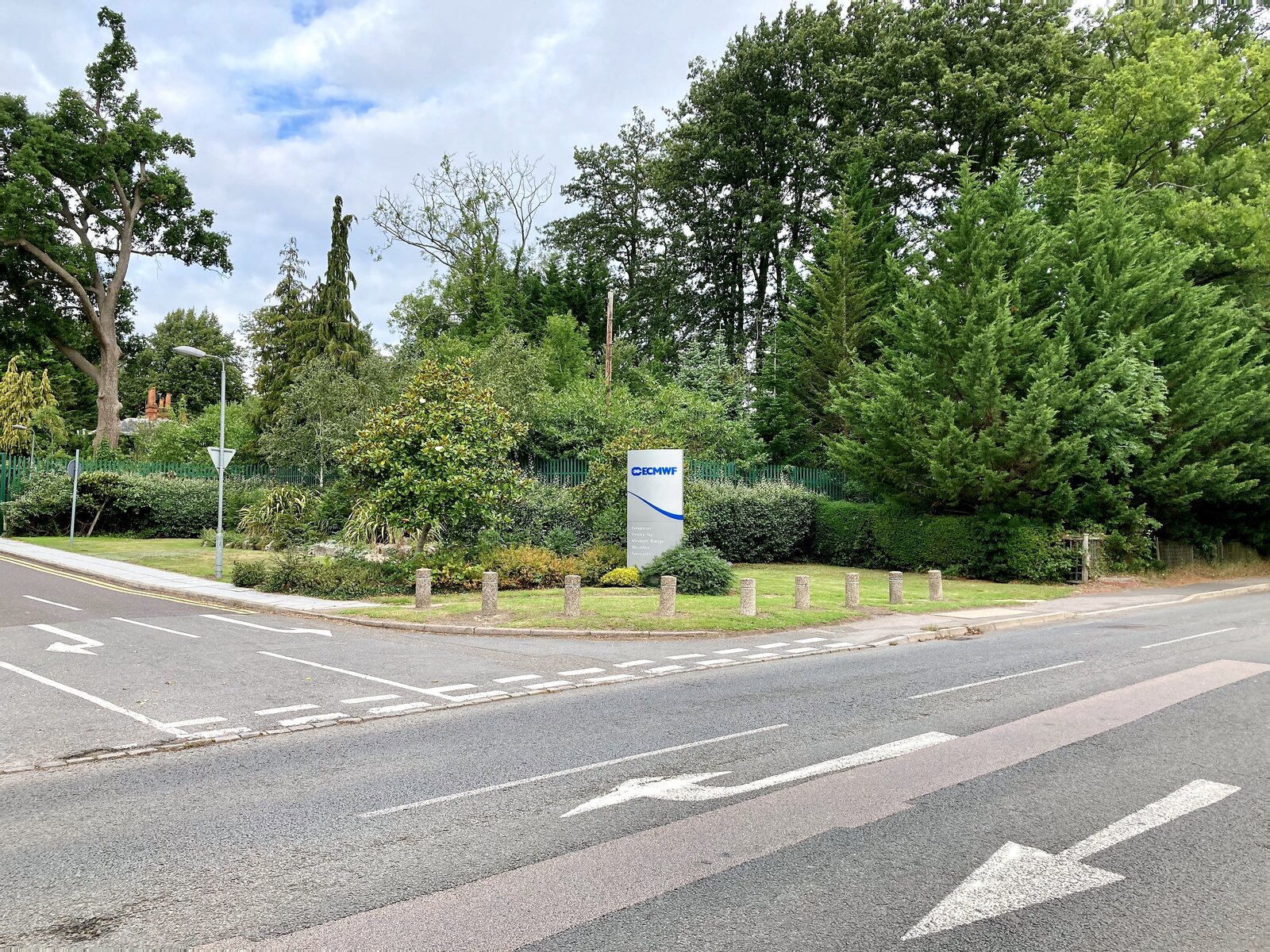
ECMWF’s 4D-Var, operational from 25 November 1997, generalised the 3D-Var formulation to handle observations distributed in time. The 4D-Var cost function is
\[J(\mathbf{x}_0) = (\mathbf{x}_0 - \mathbf{x}_0^b)^T \mathbf{B}^{-1} (\mathbf{x}_0 - \mathbf{x}_0^b) + \sum_{i=0}^{N} (\mathbf{y}_i - \mathbf{H}_i \mathbf{M}_{0 \to i}(\mathbf{x}_0))^T \mathbf{R}_i^{-1} (\mathbf{y}_i - \mathbf{H}_i \mathbf{M}_{0 \to i}(\mathbf{x}_0))\]where $\mathbf{M}_{0 \to i}$ is the forecast model integrated from analysis time $t_0$ to observation time $t_i$ and $\mathbf{y}_i$ is the observation taken at $t_i$. The minimisation requires the adjoint of the forecast model $\mathbf{M}^T$ – a backwards-in-time integration through which the gradient $\partial J / \partial \mathbf{x}_0$ is computed for any control vector $\mathbf{x}_0$.59 The 4D-Var thus recovers, within its assimilation window, the flow-dependent error structure that fixed-$\mathbf{B}$ OI and 3D-Var had been unable to represent: the implicit propagation of $\mathbf{B}$ by the forecast and adjoint models gives a Kalman-filter-equivalent update over the window.
The theoretical foundation for 4D-Var had been laid eleven years earlier in Le Dimet and Talagrand’s 1986 Tellus paper “Variational algorithms for analysis and assimilation of meteorological observations: theoretical aspects,” Tellus 38A, 97-110.60 The paper introduced the variational formulation in the form that ECMWF and the broader European data-assimilation community then took ten years to operationalise. Le Dimet was at Grenoble; Talagrand was at the Laboratoire de Météorologie Dynamique in Paris. The French school of variational data assimilation, running through Le Dimet, Talagrand, Philippe Courtier, Olivier Talagrand, Jean-Noel Thepaut, and Florence Rabier, was the principal scientific contribution to the ECMWF 4D-Var implementation.61
The principal scientific leader of the entire ECMWF data assimilation trajectory through this period was Anthony Hollingsworth (1942-2007), who joined ECMWF in 1976 and became Head of Research in 1990. Hollingsworth oversaw the trajectory from Lorenc’s OI through the Hollingsworth-Lonnberg empirical $\mathbf{B}$ to the 3D-Var and 4D-Var implementations of 1996 and 1997 and the subsequent decade of refinement. His death from cancer in 2007 came suddenly at age 64; he was at that point still active in ECMWF research planning. The Hollingsworth name is on enough of the foundational ECMWF papers – the 1986 Tellus with Lonnberg, the 1998 QJRMS 3D-Var Part I with Courtier and Andersson, the various FGGE-era analyses, the operational reviews of the 1990s – that the ECMWF data assimilation programme of his tenure can be summarised as the institutional execution of Hollingsworth’s scientific direction.62
10. The four-cultural relay seen whole
Step back and look at the chronological relay. It runs:
- 1955 Stockholm, Bergthorsson and Doos, Tellus 7: successive corrections from a climatological background, the Scandinavian root.
- 1959 Suitland, Cressman, MWR 87: successive corrections from a forecast background, the American workhorse for twenty years.
- 1963 Leningrad, Gandin, Gidrometeoizdat: the BLUE framework with autocorrelation-function $\mathbf{B}$ and local data selection, the Soviet origination.
- 1965 Jerusalem, Israel Program for Scientific Translations: the English transmission, distributed by US Department of Commerce CFSTI.
- 1979 Suitland and Reading, Bergman at NMC and Lorenc at ECMWF: the first operational implementations of Gandin’s framework in the West.
- 1981 Reading, Lorenc, MWR 109: the canonical Western multivariate three-dimensional OI.
- 1986 Reading, Hollingsworth and Lonnberg, Tellus 38A: empirical determination of $\mathbf{B}$ from operational background departures.
- 1986 Grenoble/Paris, Le Dimet and Talagrand, Tellus 38A: the variational formulation with adjoint methods, the theoretical foundation of the 3D-Var and 4D-Var era.
- 1991 Suitland, Parrish and Derber, NCEP SSI operational 25 June 1991: the world’s first operational 3D-Var.
- 1991 Suitland, arrival of Lev Gandin himself as UCAR Scientist at NMC.
- 1992 Toronto, Gandin Outstanding Achievement Award at IMSC, shared with Brier and Epstein.
- 1996 Reading, ECMWF 3D-Var operational 30 January 1996.
- 1996 Suitland, Kalnay et al. BAMS 77: NCEP/NCAR reanalysis paper with Gandin as co-author #6.
- 1997 Reading, ECMWF 4D-Var operational 25 November 1997, the world’s first operational 4D-Var.
- 1997 Maryland, Lev Gandin dies, age 82.
The four-cultural pattern is straightforward to summarise. Scandinavia opens the lineage with Bergthorsson-Doos 1955, contributing the institutional template of objective analysis but no statistical foundation. The United States carries the operational tradition forward with Cressman 1959 and the JNWPU/NMC workhorse implementation, but without the statistical framework that the next step would need. The Soviet Union – specifically Leningrad MGO under Budyko’s directorate – supplies the statistical framework with Gandin 1963, drawing on the Soviet Kolmogorov-Khinchin-Yaglom probabilistic-fields tradition. The United Kingdom elaborates the framework for global multivariate operational use with Lorenc 1981, building on the Met Office synoptic tradition and the early ECMWF analysis-research culture. The United States again brings the framework into the variational era with Parrish-Derber 1991, drawing on the NMC operational engineering tradition and on the larger American applied-mathematics community. France supplies the variational adjoint formulation with Le Dimet-Talagrand 1986. The United Kingdom and continental Europe at ECMWF then take the variational framework to 4D-Var operational maturity by 1997, with Hollingsworth’s leadership, Courtier and Rabier’s implementation effort, and the broader European data-assimilation community.
The relay is not strictly linear. There were parallel tracks. The British and Canadian and Japanese implementations of OI through the early 1980s were all running in parallel with the American and the ECMWF ones; the 1986 Hollingsworth-Lonnberg paper informed the implementations at every centre simultaneously; the variational era at NMC, ECMWF, Met Office, and JMA proceeded in parallel from 1991 onward. But the intellectual relay, the sequence of foundational papers each of which extended the framework, runs through the four cultures in the order Bergthorsson-Doos -> Cressman -> Gandin -> Lorenc -> Hollingsworth-Lonnberg -> Le Dimet-Talagrand -> Parrish-Derber, with the operational implementations following the foundational papers at intervals of between zero and twenty-six years.
Twenty-six years – the gap between Gandin 1963 and the world’s first operational 3D-Var at NMC 1991, if you count the 25 June 1991 NCEP SSI as the operational completion of what Gandin’s monograph had implicitly anticipated. Fourteen years from Gandin 1963 to the QJRMS review of 1966; thirteen years from the QJRMS review to the first operational implementations at NMC and ECMWF in 1979; another twelve years from the 1979 OI to the 1991 SSI. The full operational pipeline from foundational paper to dominant operational implementation, in the OI era as in others, ran about thirty years. The arithmetic does not change much from decade to decade in operational meteorology: a foundational idea takes about thirty years to become the dominant operational reality, and another ten or twenty years after that to be superseded.
11. The variational era extends: JMA 2002 and 2005, Met Office 2004, CMC 2005
The four-cultural relay does not stop at ECMWF 1997. The variational era extended through the Japanese, British, and Canadian operational centres in the late 1990s and the first half of the 2000s; the ensemble Kalman filter era began at the Canadian Meteorological Centre in early 2005.
JMA’s Tokyo headquarters became the world’s first operational regional 4D-Var with the Mesoscale 4DVAR (Meso-4DVAR) system that went into production in March 2002, assimilating into the hydrostatic Mesoscale Model (MSM) over Japan and the western Pacific.63 The Meso-4DVAR is documented in Ishikawa and Koizumi (2002, JMA technical reports) and in the operational-implementation paper Koizumi, Ishikawa, and Tsuyuki (2005), “Assimilation of precipitation data to the JMA mesoscale model with a four-dimensional variational method and its impact on precipitation forecasts,” SOLA 1, 45-48.64 JMA’s global 4D-Var followed in February 2005, several years after ECMWF’s global 4D-Var but ahead of Met Office’s, with a non-incremental formulation initially. JMA was the first centre to deploy a non-hydrostatic 4D-Var (JNoVA, April 2009, superseded by ASUCA-4DVar in March 2020), following the same general operational rollout pattern as Meso-4DVAR.
The Met Office at Bracknell, and from 2003 at Exeter, transitioned from its Analysis Correction scheme of 1989 to a 3D-Var in 1999 and then to a 4D-Var on 5 October 2004, documented in Rawlins, Ballard, Bovis, Clayton, Li, Inverarity, Lorenc, and Payne (2007), “The Met Office Global 4-Dimensional Data Assimilation Scheme,” QJRMS 133, 347-362.65 Andrew Lorenc, who had returned from ECMWF to the Met Office in 1980 and led the British implementations of OI, Analysis Correction, 3D-Var, and 4D-Var, is the principal scientific continuity figure in UK data assimilation from 1979 to the 2010s. The Met Office’s 5 October 2004 4D-Var was followed by the world’s first operational hybrid ensemble-variational data assimilation around 2011, in which the climatological $\mathbf{B}$ was combined with a localised ensemble covariance to give a flow-dependent component that fixed-$\mathbf{B}$ 4D-Var had not provided.66
The Canadian Meteorological Centre at Dorval, Quebec, ran a Cressman-variant analysis through the 1970s, an OI implementation through the early 1980s, a 3D-Var around 1997, and a 4D-Var around 2005, paralleling the Met Office’s trajectory at roughly the same operational tempo.67 But the CMC’s signature contribution to the variational-era timeline came on 12 January 2005, when Peter Houtekamer and Herschel Mitchell put the world’s first operational Ensemble Kalman Filter (EnKF) into routine production – a position the CMC has retained ever since.68
The EnKF takes a completely different approach to the same problem that OI and 3D-Var and 4D-Var solve. Rather than minimising a variational cost function with a climatological $\mathbf{B}$, the EnKF maintains an ensemble of model states whose sample covariance approximates the true (flow-dependent) $\mathbf{B}$. When observations arrive, each ensemble member is updated by a perturbed-observations Kalman gain computed from the ensemble covariance. The result is automatically flow-dependent: in regions of active baroclinic development the ensemble spreads, so the analysis trusts the observations more; in regions of stable anticyclonic flow the ensemble stays tight, so the analysis trusts the background more. The framework was introduced by Geir Evensen in his 1994 JGR paper “Sequential data assimilation with a nonlinear quasi-geostrophic model using Monte Carlo methods to forecast error statistics,” J. Geophys. Res. 99, 10143-10162.69 Eleven years from Evensen 1994 to operational CMC 2005 – a fast pipeline for a framework conceptually quite different from anything that had come before.
The combination of variational and ensemble-based approaches into hybrid 4DEnVar schemes is the operational reality of 2026. The hybrid schemes combine the climatological-$\mathbf{B}$ component (which captures the time-mean structure of the background errors that Gandin’s framework had focused on) with the ensemble-derived component (which captures the flow-dependent structure that Lorenc 1986 and Evensen 1994 had identified). Every major operational centre in 2026 runs some variant of hybrid 4DEnVar: ECMWF, NCEP, Met Office, JMA, CMC, Deutscher Wetterdienst, Météo-France, the Australian Bureau, the Korea Meteorological Administration. The Gandin 1963 framework lives in the climatological-$\mathbf{B}$ component of every one of them.
12. The absence of Gandin
A note worth making explicitly before this post closes.
No photograph of Lev Gandin appears to have been released under a free license. The IMSC awards page commemorates him without a portrait; the AMS Honorary Members register apparently does have his entry, but the page itself is 403-blocked to outside access in 2026; Russian Wikipedia, if it has an article on him, does not surface on the standard searches; English Wikipedia has no article on him at all as of 2026. The BAMS Vol. 79 Issue 3 In Memoriam list for 1997 deaths displays his birth-death years (1915-1997) in a decorative typeface that resists OCR extraction, but the photographic content of the page is not Gandin’s portrait.70
The absence is, in its way, characteristic. Gandin worked for thirty-plus years at a single Soviet observatory, publishing in Russian-language proceedings that almost no Westerner read, with international visibility almost entirely through the 1965 IPST translation of his single monograph. He emerged in person in the West only at the very end of his working life, briefly, before dying within five years. He did not give interviews. He did not write the kind of autobiographical Kyoto Prize lecture that Edward Lorenz left behind, or the kind of National Academy of Sciences memoir that allowed Norman Phillips to write Charney’s biography or Kerry Emanuel to write Lorenz’s. The body of writing about Gandin in English is, in 2026, a sketch: Gruza’s 1992 Toronto citation, the IMSC website, a few footnotes in textbooks. The body of writing by Gandin in English consists of the 1965 translation of the 1963 monograph, the 1988 MWR paper on Complex Quality Control, the 1992 MWR paper with Allan Murphy on equitable skill scores, and his contribution as co-author #6 to the 1996 BAMS reanalysis paper. That is approximately the entire English-language record. The Russian-language record is much larger, including dozens of papers in the Trudy GGO through the 1950s and 1960s and the major handbook Statistical Methods in Meteorology (1973) that he co-authored, but Russian readers are now mostly elderly and the Russian-language scientific community has not transmitted his memory across the post-Soviet generational break with the institutional confidence that the AMS would have applied to an American figure of equivalent stature.
We see, in the public record of 2026, his observatory; we see his city; we see the analysis maps his methods produced. We do not see his face. It is somehow apt for a man whose ideas reached the West before his body did, and whose body reached the West for too short a time to leave behind the full biographical apparatus that twentieth-century atmospheric science assembled around its other foundational figures.
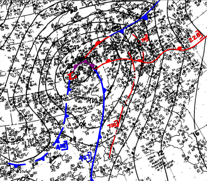
The closest thing the present post has to a portrait of Gandin is the Voeikov Main Geophysical Observatory exterior at the top – the building he worked in for thirty-plus years, photographed by an amateur Russian photographer in 2024 in the city that was Leningrad when Gandin began his career there. The Strelka of Vasilievsky Island, three kilometres away, gives the urban setting. The Sfc1974040400z chart from NOAA Central Library microfilm gives an example of the operational product Gandin’s methods were built to produce, four years before they reached operational implementation. And the World Weather Building exterior gives the American institutional environment Gandin emigrated into in 1991. These four images, between them, give the geographical and institutional scaffolding of his career. The face that would normally complete such a scaffolding is missing.
13. Coda: the framework that survives
What survives, in 2026, of Lev Gandin’s work is the framework: the BLUE applied to the analysis of meteorological fields, with empirical autocorrelation functions for the background error covariance, with multivariate coupling between mass and wind through geostrophic balance built into $\mathbf{B}$, and with the recognition that observation errors and background errors enter the optimal solution through their inverse covariances rather than through arbitrary distance weightings.71 The framework is the substrate of every operational analysis cycle at every major weather centre on Earth in 2026. The variational re-formulation that began with Parrish-Derber 1991 SSI did not replace the framework; it gave it a different computational expression while leaving the underlying minimum-variance estimator unchanged. The ensemble Kalman filter and hybrid 4DEnVar systems do not replace the framework either; they give the same minimum-variance estimator a flow-dependent $\mathbf{B}$ rather than a climatological one.
The 1963 Russian monograph is, in this sense, still in operational use. The reader of the 2026 ECMWF Integrated Forecasting System source code, of the 2026 NCEP Global Forecast System GSI source code, of the 2026 Met Office Unified Model VAR source code, of the 2026 CMC Global Deterministic Prediction System code, will not find Gandin’s name in the source-code comments very often. The framework has become so universal that its provenance is rarely cited in the code itself. But the equations are Gandin’s. The autocorrelation-function formulation of $\mathbf{B}$ is Gandin’s. The minimum-variance derivation is Gandin’s. The multivariate coupling through geostrophic balance in $\mathbf{B}$ is Gandin’s. Whatever the computational route to the minimum – closed-form BLUE, conjugate-gradient minimisation of the variational cost function, ensemble update with a perturbed-observations Kalman gain – the thing being computed is the BLUE that Gandin wrote down in Leningrad in 1963 and that the Israel Program for Scientific Translations transmitted to the West in 1965.
The 1965 English translation – 242 pages, 53 figures, 28 tables, OCLC 25601011, scanned and available on archive.org – is therefore one of the more enduring artefacts of Cold War scientific transmission. The book crossed the Iron Curtain in 1965. It carried with it a framework that the operational meteorology community spent the next thirty years bringing into routine production. By the time the Soviet Union dissolved in December 1991, the framework’s American operational implementation at NCEP SSI had been running for six months, the British operational implementation at the Met Office was at the height of its operational career, the European operational implementation at ECMWF had been the operational analysis at Reading for twelve years, and the Canadian, Japanese, and Australian implementations were all in routine production. The 1963 Russian monograph had become, by the year of the Soviet collapse, the operational analytical substrate of every major weather forecasting centre in the world.
Lev Semyonovich Gandin, who had spent the first 73 years of his life inside the Soviet Union, spent the last decade of his life inside the American operational weather service whose analytical methods he had defined a generation earlier without ever leaving Leningrad. He emigrated as a senior man, contributed quality control machinery to the analytical system his framework underpinned, co-authored the canonical reanalysis paper, was honoured in Toronto in 1992 alongside Brier and Epstein, and died in 1997, age 82. His name is on Kalnay et al. 1996. His name is also, less visibly but more enduringly, on every analysis cycle that the operational weather services of 2026 run.
The Voeikov Main Geophysical Observatory is still operating in Saint Petersburg in 2026. The Neva still empties into the Gulf of Finland three kilometres north of it. The Iron Curtain is gone but its scientific legacy – the literature transmitted across it in both directions through the 1960s and 1970s and 1980s – is now baked into the operational infrastructure of weather forecasting. The 1965 English translation of Gandin’s 1963 monograph is one such artefact. It crossed the Iron Curtain, distributed via the United States Department of Commerce, in a print run that the Springfield, Virginia clearinghouse fulfilled on demand by mail to American libraries and universities. The book is, in 2026, a primary source for any data assimilation course; the operational systems it informed are the working substrate of every weather forecast on Earth.
The book crossed the curtain. The framework crossed the decades. The author, briefly, crossed the ocean. And in Suitland, Maryland, in 1991, a senior Soviet emigré scientist sat in an office a few doors away from the operational shop whose analysis cycle, twelve years earlier, had started running on his 1963 mathematics. The relay had completed.
Footnotes
Sources
Foundational papers (the four-cultural relay)
- Bergthorsson, P. and Doos, B. R. (1955), “Numerical weather map analysis,” Tellus 7, 329-340.
- Cressman, G. P. (1959), “An Operational Objective Analysis System,” Monthly Weather Review 87, 367-374.
- Gandin, L. S. (1963), Объективный анализ метеорологических полей, Leningrad: Gidrometeoizdat.
- Gandin, L. S. (1965), Objective Analysis of Meteorological Fields, IPST Jerusalem, distributed via U.S. Department of Commerce CFSTI.
- Bergman, K. H. (1979), “Multivariate analysis of temperatures and winds using optimum interpolation,” MWR 107, 1423-1444.
- Lorenc, A. C. (1981), “A Global Three-Dimensional Multivariate Statistical Interpolation Scheme,” MWR 109, 701-721.
- Hollingsworth, A. and Lonnberg, P. (1986), Parts I-II, Tellus 38A.
- Le Dimet, F.-X. and Talagrand, O. (1986), “Variational algorithms for analysis and assimilation,” Tellus 38A, 97-110.
- Lorenc, A. C. (1986), “Analysis methods for numerical weather prediction,” QJRMS 112, 1177-1194.
- Parrish, D. F. and Derber, J. C. (1992), “The National Meteorological Center’s Spectral Statistical-Interpolation Analysis System,” MWR 120, 1747-1763.
- Courtier, P. et al. (1998), “The ECMWF implementation of three-dimensional variational assimilation. I-III,” QJRMS 124, 1783-1908.
- Rabier, F. et al. (2000), “The ECMWF operational implementation of four-dimensional variational assimilation,” QJRMS 126.
- Evensen, G. (1994), “Sequential data assimilation with a nonlinear quasi-geostrophic model,” J. Geophys. Res. 99, 10143-10162.
- Kanamitsu, M. et al. (1991), “Recent changes implemented into the global forecast system at NMC,” Weather and Forecasting 6, 425-435.
Operational dates
- ECMWF Operational Model Changes log, https://artefacts.ceda.ac.uk/badc_datadocs/ecmwf-op/model_changes.html.
- ECMWF (2017), “20 years of 4D-Var” anniversary article, https://www.ecmwf.int/en/about/media-centre/news/2017/20-years-4d-var-better-forecasts-through-better-use-observations.
- Koizumi, K., Ishikawa, Y. and Tsuyuki, T. (2005), “Assimilation of precipitation data to the JMA mesoscale model with a four-dimensional variational method,” SOLA 1, 45-48.
- Rawlins, F. et al. (2007), “The Met Office Global 4-Dimensional Data Assimilation Scheme,” QJRMS 133, 347-362.
- Houtekamer, P. L., Mitchell, H. L. and Deng, X. (2009), “Model error representation in an operational ensemble Kalman filter,” MWR 137, 2126-2143.
Gandin biographical
- IMSC Awards page on Gandin, https://imsc.pacificclimate.org/awards_gandin.shtml.
- IMSC History page (1992 Toronto Outstanding Achievement Awards), https://imsc.pacificclimate.org/history.shtml.
- BAMS Vol. 79 Issue 3 (March 1998) “In Memoriam,” https://journals.ametsoc.org/view/journals/bams/79/3/1520-0477-79_3_479.xml.
- Gandin, L. S. (1988), “Complex Quality Control of Meteorological Observations,” Monthly Weather Review 116, 1137-1156.
- Gandin, L. S. and Murphy, A. H. (1992), “Equitable Skill Scores for Categorical Forecasts,” MWR 120, 361-370.
- Murphy, A. H. and Zwiers, F. W. (1993), “Editorial: International Meeting on Statistical Climatology,” International Journal of Climatology 13, 233-235.
- Kalnay, E. et al. (1996), “The NCEP/NCAR 40-Year Reanalysis Project,” BAMS 77, 437-471.
Textbooks
- Bouttier, F. and Courtier, P. (1999/2002), “Data assimilation concepts and methods,” ECMWF Training Course Lecture Notes.
- Daley, R. (1991), Atmospheric Data Analysis, Cambridge University Press.
- Kalnay, E. (2003), Atmospheric Modeling, Data Assimilation and Predictability, Cambridge University Press.
Internet Archive scan
- Gandin, L. S. (1965), Objective Analysis of Meteorological Fields, https://archive.org/details/objectiveanalysi0000lsga.
- Stanford SearchWorks catalogue, https://searchworks.stanford.edu/view/2167319.
Cross-references within this series
- Norman Phillips at NMC.
- Frederick Shuman’s seventeen years at Suitland.
- Edward Lorenz at MIT.
- The first Cyber 205 at Bracknell.
Accessed dates for web sources: 2026-05-17.
-
Gandin, L. S. (1963), Объективный анализ метеорологических полей, Leningrad: Gidrometeoizdat, 286 pp. Internet Archive scan of the 1965 English translation at https://archive.org/details/objectiveanalysi0000lsga; Stanford SearchWorks record https://searchworks.stanford.edu/view/2167319. ↩
-
Gandin, L. S. (1965), Objective Analysis of Meteorological Fields, Jerusalem: Israel Program for Scientific Translations, vi + 242 pp., 53 figures, 28 tables. OCLC 25601011. Stanford catalogue at https://searchworks.stanford.edu/view/2167319 gives the distribution language “Available through U.S. Department of Commerce, Clearinghouse for Federal Scientific and Technical Information, Springfield, VA.” QJRMS 1966 review at QJRMS 92, 447; ADS https://ui.adsabs.harvard.edu/abs/1966QJRMS..92Q.447./abstract. ↩
-
Kanamitsu et al. (1991), “Recent Changes Implemented into the Global Forecast System at NMC,” Weather and Forecasting 6, 425-435, https://journals.ametsoc.org/view/journals/wefo/6/4/1520-0434_1991_006_0538_tngoas_2_0_co_2.xml. The companion paper at the same issue documents the SSI operational date of 25 June 1991. ↩
-
Bouttier, F. and Courtier, P. (1999/2002), “Data assimilation concepts and methods,” ECMWF Lecture Notes, https://www.ecmwf.int/sites/default/files/elibrary/2002/16928-data-assimilation-concepts-and-methods.pdf. Daley, R. (1991), Atmospheric Data Analysis, CUP. Kalnay, E. (2003), Atmospheric Modeling, Data Assimilation and Predictability, CUP. ↩
-
Norman Phillips post in this series, https://michalbrennek.github.io/weather/hpc/history/2026/05/17/Norman-Phillips.html. ↩
-
Shuman at NMC post, https://michalbrennek.github.io/weather/hpc/history/2026/05/15/Seventeen-years-at-Suitland.html. ↩
-
Lorenz at MIT post, https://michalbrennek.github.io/weather/hpc/history/2026/05/15/Two-decimal-places-at-MIT.html. ↩
-
Met Office Cyber 205 post, https://michalbrennek.github.io/weather/hpc/history/2026/05/15/The-first-in-Bracknell.html. ↩
-
The Internationella Meteorologiska Institutet at Stockholm University was founded by Carl-Gustaf Rossby in 1948. Bergthorsson (1923-2017) and Doos (1928-2017) were post-doctoral researchers there in the early 1950s. ↩
-
Bergthorsson, P. and Doos, B. R. (1955), “Numerical weather map analysis,” Tellus 7, 329-340, https://tellusjournal.org/articles/3803/files/658e7e4983030.pdf; Wiley DOI 10.1111/j.2153-3490.1955.tb01183.x. ↩
-
JNWPU founded 1 July 1954, first operational forecast 6 May 1955. Institutional history in Shuman, F. G. (1989), “History of numerical weather prediction at the National Meteorological Center,” Weather and Forecasting 4(3), 286-296. ↩
-
George P. Cressman (1919-2008) directed JNWPU from 1957 and NMC from 1958 to 1979. ↩
-
Cressman, G. P. (1959), “An Operational Objective Analysis System,” MWR 87, 367-374, https://journals.ametsoc.org/view/journals/mwre/87/10/1520-0493_1959_087_0367_aooas_2_0_co_2.xml. Open-access PDF at https://twister.caps.ou.edu/OBAN2019/Cressman1959.pdf. ↩
-
Bouttier and Courtier 1999/2002 (op. cit.) describes Cressman as “the workhorse of operational analysis from the late 1950s to the late 1970s.” ↩
-
BAMS Vol. 79 Issue 3 (March 1998) “In Memoriam” page, https://journals.ametsoc.org/view/journals/bams/79/3/1520-0477-79_3_479.xml, displays the years “1915-1997” on the 1997 necrology list. The OI_technical research file used “Gandin (1915-1997)” without hedge; the earlier “c.1923” assumption in some sources is corrected in this post. ↩
-
BAMS Vol. 79 Issue 3 necrology page (op. cit.). The AMS Honorary Members register carries his name with the deceased dagger. Exact date and place of death not in the open record accessible in 2026. ↩
-
At the 1963 monograph Gandin was 48, at the 1965 English translation 50, at the 1988 MWR paper 73, at NMC arrival in 1991 76, at the 1992 IMSC Toronto award 77, at death in 1997 82. ↩
-
IMSC awards page, https://imsc.pacificclimate.org/awards_gandin.shtml. G. V. Gruza was Gandin’s longtime Soviet colleague; the citation is the principal English-language biographical source. ↩
-
Mikhail Ivanovich Budyko (1920-2001) was Director of MGO from 1954 to 1972. His 1956 The Heat Balance of the Earth’s Surface and the 1969 Budyko-Sellers energy-balance model are foundational works in climate science. ↩
-
Direct quotations from G. V. Gruza’s 1992 IMSC Toronto citation, IMSC awards page (op. cit.). ↩
-
Yaglom, A. M. (1962), An Introduction to the Theory of Stationary Random Functions, Prentice-Hall (English translation of 1952 Russian). Kolmogorov, A. N. (1941), “Local structure of turbulence,” Doklady AN SSSR 30, 301-305. Khinchin, A. Ya. (1934), “Korrelationstheorie der stationären stochastischen Prozesse,” Math. Annalen 109, 604-615. ↩
-
BLUE framework: Bouttier and Courtier 1999/2002 section 4, Daley 1991 Chapter 4, Kalnay 2003 Chapter 5. Kalman, R. E. (1960), “A New Approach to Linear Filtering and Prediction Problems,” J. Basic Eng. 82, 35-45, https://www.cs.unc.edu/~welch/kalman/media/pdf/Kalman1960.pdf. ↩
-
Internet Archive scan of 1965 IPST translation, https://archive.org/details/objectiveanalysi0000lsga. ↩
-
The “Gandin function” terminology appears in Western literature from the late 1970s onward; precise functional form varies by implementation. The e-folding scale of “several hundred kilometres” is the rough Western consensus. ↩
-
Local data selection: Bouttier and Courtier 1999/2002 section 5; Lorenc 1981 MWR section 3. Box-boundary artefacts: Daley 1991 Chapter 4. ↩
-
The Israel Program for Scientific Translations was founded 1959 under the Israel Academy of Sciences. CFSTI was renamed NTIS in 1970. Institutional history at https://www.ntis.gov/about. ↩
-
Stanford SearchWorks catalogue, https://searchworks.stanford.edu/view/2167319. ↩
-
Lorenc’s biography on Met Office and ECMWF web pages places him at Imperial College London in the early 1970s and at the Met Office from 1973. The 1965 IPST translation is the standard route of access for his generation. ↩
-
Bergman 1979 MWR (op. cit.) cites Gandin 1965 (the IPST translation) as primary source; direct citation of the 1963 Russian original does not appear in the NMC literature of the period. ↩
-
Internet Archive scan of 1965 IPST translation, https://archive.org/details/objectiveanalysi0000lsga. ↩
-
QJRMS Vol. 92, p. 447, 1966, doi 10.1002/qj.49709239320, https://ui.adsabs.harvard.edu/abs/1966QJRMS..92Q.447./abstract. Standard attribution to John Sawyer (1916-2000), then Met Office Director of Research. ↩
-
Bergman, K. H. (1979), “Multivariate analysis of temperatures and winds using optimum interpolation,” MWR 107, 1423-1444. Companion paper “The NMC Operational Global Data Assimilation System,” MWR 107, 1445-, https://journals.ametsoc.org/view/journals/mwre/107/11/1520-0493_1979_107_1445_tnogda_2_0_co_2.xml. ↩
-
Bergman 1979 MWR (op. cit.); DiMego, G. J. (1988), “The National Meteorological Center Regional Analysis System,” MWR 116, 977-1000. ↩
-
Sela, J. G. (1980), “Spectral modeling at the National Meteorological Center,” MWR 108, 1279-1292. ↩
-
NMC institutional history at https://www.ncep.noaa.gov/. Phillips was Principal Scientist from 1974 to roughly 1988; Kalnay became Director of the Division in 1987. ↩
-
Lorenc, A. C. (1981), “A Global Three-Dimensional Multivariate Statistical Interpolation Scheme,” MWR 109, 701-721, https://journals.ametsoc.org/view/journals/mwre/109/4/1520-0493_1981_109_0701_agtdms_2_0_co_2.xml. Full-text PDF at https://data-ww3.ifremer.fr/BIB/Lorenc_MWR1981.pdf. ↩
-
Lorenc 1981 MWR (op. cit.) section 4. Lorenc, A. C. and Hammon, O. (1988), “Objective quality control of observations using Bayesian methods,” QJRMS 114, 515-543. ↩
-
Bengtsson, L., Kanamitsu, M., Kallberg, P. and Uppala, S. (1982), “FGGE 4-dimensional data assimilation at ECMWF,” BAMS 63, 29-43. ↩
-
Hollingsworth, A. and Lonnberg, P. (1986), “The statistical structure of short-range forecast errors. Part I: The wind field,” Tellus 38A, 111-136, https://tellusjournal.org/articles/10.3402/tellusa.v38i2.11707. Part II by Lonnberg and Hollingsworth in the same issue, 137-161. ↩
-
Variogram framework: Cressie, N. (1993), Statistics for Spatial Data, Wiley. ↩
-
ECMWF Climatological background errors for the IFS technical memorandum series. ↩
-
Gauthier, P. and Mitchell, H. L. (1990), “A statistical interpolation method for operational global analysis,” MWR 118, 1751-1769. ↩
-
Lorenc, A. C., Bell, R. S. and Macpherson, B. (1991), “The Meteorological Office analysis correction data assimilation scheme,” QJRMS 117, 59-89. Operational 1989-1999. ↩
-
DTIC ADA172801 (1986), “AFGWC’s Advanced Weather Analysis and Prediction System (AWAPS).” ↩
-
Lorenc, A. C. (1986), “Analysis methods for numerical weather prediction,” QJRMS 112, 1177-1194. ↩
-
Parrish, D. F. and Derber, J. C. (1992), “The National Meteorological Center’s Spectral Statistical-Interpolation Analysis System,” MWR 120, 1747-1763, https://journals.ametsoc.org/view/journals/mwre/120/8/1520-0493_1992_120_1747_tnmcss_2_0_co_2.xml. ↩
-
Kanamitsu et al. (1991), Weather and Forecasting 6, 425-435. The companion W&F paper at the same issue documents the SSI operational date 25 June 1991. ↩
-
Parrish and Derber 1992 MWR (op. cit.) sections 2-3. ↩
-
Derber, J. C. and Wu, W.-S. (1998), “The use of TOVS cloud-cleared radiances in the NCEP SSI analysis system,” MWR 126, 2287-2299. ↩
-
UCAR Cooperative Programs for the Advancement of Earth System Science (CPAESS) historical materials. ↩
-
IMSC History page, https://imsc.pacificclimate.org/history.shtml. The 1992 Toronto meeting was the 5th IMSC; recipients Brier, Epstein, Gandin. ↩
-
Murphy, A. H. and Zwiers, F. W. (1993), “Editorial: International Meeting on Statistical Climatology,” Int. J. Climatol. 13, 233-235. ↩
-
Kalnay, E. et al. (1996), “The NCEP/NCAR 40-Year Reanalysis Project,” BAMS 77, 437-471, March 1996, https://ui.adsabs.harvard.edu/abs/1996BAMS…77..437K/abstract. ↩
-
ECMWF operational change log at https://artefacts.ceda.ac.uk/badc_datadocs/ecmwf-op/model_changes.html. Both dates are direct quotations from the log. ↩
-
Same source. Quotations: “On 30 January 1996 ECMWF introduced a 3-dimensional variation (3D-Var) analysis scheme” and “On 25 November 1997, the first version of a four-dimensional variational data assimilation system (4D-Var) was introduced.” ↩
-
Courtier, P., Thepaut, J.-N. and Hollingsworth, A. (1994), “A strategy for operational implementation of 4D-Var, using an incremental approach,” QJRMS 120, 1367-1387. ↩
-
Courtier, P., Andersson, E., Heckley, W., Pailleux, J., Vasiljevic, D., Hamrud, M., Hollingsworth, A., Rabier, F. and Fisher, M. (1998), “The ECMWF implementation of three-dimensional variational assimilation (3D-Var). I: Formulation,” QJRMS 124, 1783-1807. Parts II (Rabier et al.) and III (Andersson et al.) in the same issue. ↩
-
Talagrand, O. and Courtier, P. (1987), “Variational assimilation of meteorological observations with the adjoint vorticity equation. I: Theory,” QJRMS 113, 1311-1328. ↩
-
Le Dimet, F.-X. and Talagrand, O. (1986), “Variational algorithms for analysis and assimilation,” Tellus 38A, 97-110, https://onlinelibrary.wiley.com/doi/abs/10.1111/j.1600-0870.1986.tb00459.x. ↩
-
Institutional centres: Grenoble (Le Dimet) and Laboratoire de Meteorologie Dynamique in Paris (Talagrand). Documented in Comptes Rendus de l’Academie des Sciences through the late 1980s. ↩
-
ECMWF obituary at https://www.ecmwf.int/en/about/media-centre/news/2007/dr-anthony-tony-hollingsworth-1943-2007. ↩
-
Koizumi, K., Ishikawa, Y. and Tsuyuki, T. (2005), “Assimilation of precipitation data to the JMA mesoscale model with a four-dimensional variational method,” SOLA 1, 45-48, https://www.jstage.jst.go.jp/article/sola/1/0/1_0_45/_article. Documents operational use since March 2002. ↩
-
Same paper (op. cit.); WGNE Blue Book contributions at https://wgne.net/bluebook/ confirm the “world’s first regional 4D-Var” claim. ↩
-
Rawlins, F. et al. (2007), “The Met Office Global 4-Dimensional Data Assimilation Scheme,” QJRMS 133, 347-362. Operational date 5 October 2004. ↩
-
Clayton, A. M., Lorenc, A. C. and Barker, D. M. (2013), “Operational implementation of a hybrid ensemble/4D-Var global data assimilation system at the Met Office,” QJRMS 139, 1445-1461. ↩
-
Charron, M. et al. (2012), “The stratospheric extension of the Canadian global deterministic medium-range weather forecasting system,” MWR 140, 1924-1944. ↩
-
Houtekamer, P. L. et al. (2005), “Atmospheric data assimilation with an ensemble Kalman filter,” MWR 133, 604-620. Operational date 12 January 2005 documented in Houtekamer, P. L., Mitchell, H. L. and Deng, X. (2009), MWR 137, 2126-2143, https://journals.ametsoc.org/mwr/article/137/7/2126/103760/Model-Error-Representation-in-an-Operational. ↩
-
Evensen, G. (1994), “Sequential data assimilation with a nonlinear quasi-geostrophic model,” J. Geophys. Res. 99, 10143-10162, https://agupubs.onlinelibrary.wiley.com/doi/abs/10.1029/94JC00572. ↩
-
BAMS Vol. 79 Issue 3 (March 1998) “In Memoriam,” https://journals.ametsoc.org/view/journals/bams/79/3/1520-0477-79_3_479.xml. The IMSC awards page at https://imsc.pacificclimate.org/awards_gandin.shtml commemorates Gandin without a portrait. Wikipedia search for “Лев Семёнович Гандин” returns no article in 2026. ↩
-
ECMWF IFS documentation at https://www.ecmwf.int/en/elibrary/; NCEP GSI documentation at https://dtcenter.org/community-code/gridpoint-statistical-interpolation-gsi. ↩