The Hemisphere That Caught Up

One chart shows up in almost every talk on the history of weather forecasting. The horizontal axis is the calendar, 1980 to now. The vertical axis is forecast skill – usually the anomaly correlation (a 0-to-1 score for how well the forecast reproduces the observed pattern of departures from the climatological normal) of the five-day forecast of 500 hPa geopotential height, the roughly-five-and-a-half-kilometre level that is the workhorse diagnostic of the mid-latitude circulation. Two curves climb across it. The upper one is the Northern Hemisphere, the lower one the Southern. For fifteen years they run in parallel, the South trailing the North by a wide and stubborn margin – close to a full day of predictability, so a five-day forecast in the South was worth about what a six-day forecast was worth in the North. Then, across the late 1990s and early 2000s, the lower curve bends up and closes on the upper one. By the mid-2000s they nearly touch.¹²

That convergence is one of the quiet triumphs of twentieth-century geophysics, and it has one principal cause. The South did not suddenly grow radiosonde networks and airport wind reports to rival Europe and North America. It never will; most of the Southern Hemisphere is water and ice. What happened instead is that the weather centres learned to pull from satellite radiation most of the information the sparse Northern network had been handing them for free. The satellites had flown since the 1970s. The instruments were not the thing that changed. The mathematics was. Forecasters stopped inverting radiances into temperature profiles and feeding those profiles in as though they were radiosondes, and started assimilating the raw radiances directly, with a physics model of how radiation leaves the atmosphere placed inside the analysis itself.

This is the observation side of the forecast revolution. The companion story – how the analysis engine itself changed, from the statistical interpolation of the 1970s and 1980s to the variational methods of the 1990s – ran through Post 47 of this series, which followed four-dimensional variational assimilation to its operational switch at the European Centre for Medium-Range Weather Forecasts on 25 November 1997.³ The two are inseparable: direct radiance assimilation was the first great customer of the variational machinery. But this one runs along a different axis. Not the analysis method, the observing system – and above all the satellites. How a hemisphere caught up.

1. The two curves meet

The convergence is documented in a single paper, and it is the same one that anchored Post 47: Adrian Simmons and Anthony Hollingsworth, “Some aspects of the improvement in skill of numerical weather prediction,” in the Quarterly Journal of the Royal Meteorological Society, 2002.¹ They tabulated the skill of the medium-range forecast of mean-sea-level pressure and 500 hPa height in both hemispheres, across three of the major global systems, back to about 1980. One sentence in their abstract is the sentence this whole post exists to explain:

The improvement amounts to about a one-day gain in predictability of mean-sea-level pressure and 500hPa height over the last decade in the northern hemisphere, with a similar gain over the last three years in the southern hemisphere.

The asymmetry is the crux. In the North, the one-day gain in predictability was spread over a decade of grinding, incremental progress. In the South, the same gain arrived in three years. Something in the late 1990s and early 2000s compressed a decade of Northern work into a third of the time. Later in the paper they spell out the consequence:

One-day forecast errors have been reduced so much in the southern hemisphere that medium-range forecasts for the region have become almost as skilful as those for the northern hemisphere.¹

“Almost as skilful as those for the northern hemisphere.” That is the payoff. For the whole prior history of numerical weather prediction the Southern forecast had been the perennial laggard. By the millennium the gap had all but closed. Thirteen years later Peter Bauer, Alan Thorpe and Gilbert Brunet reprinted the two converging curves as the opening figure of their Nature review “The quiet revolution of numerical weather prediction,” and the near-coincidence of the two anomaly-correlation curves became the single most reproduced image in the field.² ECMWF’s headline verification score today – the lead time at which the high-resolution forecast’s 500 hPa anomaly correlation drops through 80% – reaches nearly the same value in both hemispheres. The curves sit one on top of the other where they once stood a day apart.⁴

The cause has been tested directly, by a crude but decisive method: take the satellites away and watch. Run the ECMWF assimilation system with no satellite data and the North degrades but survives. The South collapses. A 2013 ECMWF review of satellite-data impact put it flatly – without satellite observations the loss “would still cause catastrophic degradation in the southern hemisphere, and very significant degradation in the northern hemisphere.”⁵ That gap closed after 2000, and it would reopen the instant the satellites went dark. To see why the South was ever so far behind, start with the map of where the world takes its measurements.

2. Why the Southern Hemisphere was blind

Every forecast begins with an analysis: a picture of the atmosphere at one instant, built by combining a short-range forecast – the “background,” or “first guess” – with whatever observations have arrived since the last one. The quality of that analysis, and of the forecast growing out of it, rides on the density and accuracy of the observations. And the twentieth-century observing network was built where the people were.

Take the backbone of the pre-satellite system, the radiosonde. A balloon lofts an instrument package twice a day, at 0000 and 1200 UTC, from somewhere between a few hundred and a thousand stations worldwide; it rises through the troposphere and lower stratosphere and radios back temperature, humidity, pressure and – through tracking – wind, all the way up. It is the gold standard: a vertical profile of the state variables themselves, measured in place. But radiosondes launch from land, from national weather services, near where they are needed for aviation and public forecasting. Their geography is the geography of the populated, land-heavy North – dense across Europe, North America, European Russia, China, India, Japan, and sparse to absent across the great Southern oceans.

To an observing network, the Southern Hemisphere is a different planet. Roughly four-fifths ocean. Its land is Antarctica – a continent of a few dozen research stations – the southern cones of South America and Africa, and Australia and New Zealand. Between them lie thousands of kilometres of Southern Ocean, the roaring forties and furious fifties, a band of open water round the globe where the storm tracks run hardest and the observing stations run out. A cyclone deepening in the South Pacific in 1985 could live its whole life without a single radiosonde, ship report or aircraft observation touching it. The analysis over such a region was the short-range forecast, lightly nudged by a handful of scattered surface reports – a first guess with almost nothing to pull it back toward reality.

The other conventional platforms shared the same northern bias. Commercial aircraft reported temperature and wind along their cruise tracks; those tracks thickened over the North Atlantic and North Pacific corridors and thinned to nothing over the Southern Ocean. Ships of opportunity radioed surface pressure and temperature along the shipping lanes, which again clustered in the North and along a few Southern trade routes, leaving the high southern latitudes nearly empty. Drifting buoys, deployed in growing numbers from the 1980s, gave surface pressure over the open ocean and were one of the few platforms with a real Southern presence – but they measured only at the surface, not the vertical profile the analysis most needed. The Global Observing System was, before the satellites, two systems stitched together at the equator: a dense, multi-platform, vertically-resolved network in the North, and in the South a scatter of surface reports over a hemisphere of water. The First GARP Global Experiment of 1978-79, the first coordinated attempt to observe the whole globe at once and the empirical basis for a generation of data-denial studies, was mounted for exactly this reason – the routine network left so much of the planet, and especially the South, so thinly sampled.⁶

Here the observing desert meets the deepest result in the theory of forecasting. In 1963, working at MIT on a stripped-down model of convection, Edward Lorenz found that deterministic atmospheric systems show sensitive dependence on initial conditions: two states of the atmosphere differing by too little to measure will, given time, diverge into entirely different weather. That discovery – the subject of Post 41 of this series – set a hard horizon on predictability and made the accuracy of the initial condition the master variable of forecast skill.⁷ In a data desert it cuts cruelly. Where the analysis is poorly constrained, its errors are large; where the errors are large, the forecast diverges faster; so the region that starts with the worst analysis loses its skill first. The South paid twice: a worse initial condition, amplified by the same chaos that governed the well-observed North.

The deficit was measured early and often, by the data-denial experiment: run the analysis with and without a class of observation, and compare the forecasts. The very first such experiments, on data from the 1978-79 GARP experiment, showed the pattern. When Gilchrist and colleagues withheld the space-based observations from a reanalysis of that period, useful predictability in the North fell by about a day, from roughly five and a half days to four and a half. In the South it fell by two full days, from about five to three.⁶ Even then the South leaned on the satellites for something like two days of its skill – yet the satellites of the 1970s and 1980s were not being used well enough to close the gap. Why not? Look at what a satellite sounder actually measures. It is not temperature.

3. The first eyes: what a sounder sees

A weather satellite in a polar, sun-synchronous orbit circles pole to pole at 800 to 850 kilometres while the Earth turns beneath it, crossing the equator at the same local solar time on every pass. It carries instruments that stare down and measure radiation. Here is the fact from which every difficulty and every triumph in this story descends: a passive sounder does not measure temperature, or humidity, or wind. It measures radiance – the intensity of electromagnetic radiation, at a set of chosen wavelengths, arriving from the scene below. Radiance is usually re-expressed as a brightness temperature, the temperature a perfect blackbody would need in order to emit that much radiation at that wavelength. But the quantity underneath is a measured intensity, not a measured temperature.⁶

One such satellite circles the Earth about fourteen times a day. Because the planet turns beneath it, each orbit’s swath falls to the west of the last, so in twenty-four hours the scan tiles the whole globe twice – once up the daylit side of each orbit, once down the night side. Two satellites, phased to cross the equator at different local times, sample every point on Earth four times a day. No ground network can match that. Not accuracy at a single point, where a radiosonde beats a sounder easily, but uniform global coverage, pole to pole and ocean to ocean, on a fixed daily schedule. The sounders gave up the vertical sharpness and the direct measurement of the radiosonde for something no balloon could offer: the whole planet, every day, including the four-fifths of the South no balloon would ever reach.⁶⁸

Turning radiance into knowledge of the atmosphere takes physics. The atmosphere is semi-transparent: it emits radiation according to its temperature, through Planck’s law, and absorbs according to its composition, and the balance of the two along the path to the satellite fixes what the instrument sees. The key idea is the weighting function – and here it helps to drop the symbols and picture a bank of fog. Thick fog, and you see only its near face; thin fog, and you see deep in. Each channel of a sounder looks into the atmosphere through a “fog” whose thickness is set by how strongly the air absorbs at that channel’s wavelength. A channel tuned to the strongly absorbing centre of a gas band looks into thick fog: all its radiation comes from high up, because anything from below is absorbed before it can escape. A channel tuned to the weakly absorbing wing of the same band looks into thin fog and sees deep, down toward the surface. The profile of where each channel’s signal comes from – formally, the rate of change of atmospheric transmittance with height – is that channel’s weighting function, a hump that peaks at some altitude and falls away above and below.⁶

So the trick of sounding is to pick a set of channels across an absorption band whose weighting functions peak at a staircase of altitudes. Stack them, and you have a crude set of overlapping vertical samples of the atmosphere’s emission – and from those, in principle, a temperature profile. One condition: to read temperature you must sound in a band of a gas whose concentration you already know, so a change in radiance can be pinned on a change in temperature rather than in the amount of gas. Nature obliges. Carbon dioxide is well mixed and nearly uniform through the lower atmosphere, with strong infrared bands near 15 and 4.3 micrometres. Molecular oxygen is likewise uniform, with an absorption complex near 50 to 60 gigahertz in the microwave. Temperature sounders work the carbon-dioxide and oxygen bands. Humidity is sounded in the water-vapour bands – near 6.3 micrometres in the infrared, near 183 gigahertz in the microwave – where the absorbing gas is itself the unknown being sought.⁶

The lineage of United States polar-orbiting operational satellites from TIROS-N (launched 13 October 1978) through NOAA-16. Each carried a version of the sounding suite that this post follows: TOVS on TIROS-N through NOAA-14, then ATOVS from NOAA-15 onward. The instruments barely changed in appearance across two decades; what changed was the mathematics of how their radiances were used. Illustration: NOAA, NOAA In Space Collection (spac0557), 2002, public domain.

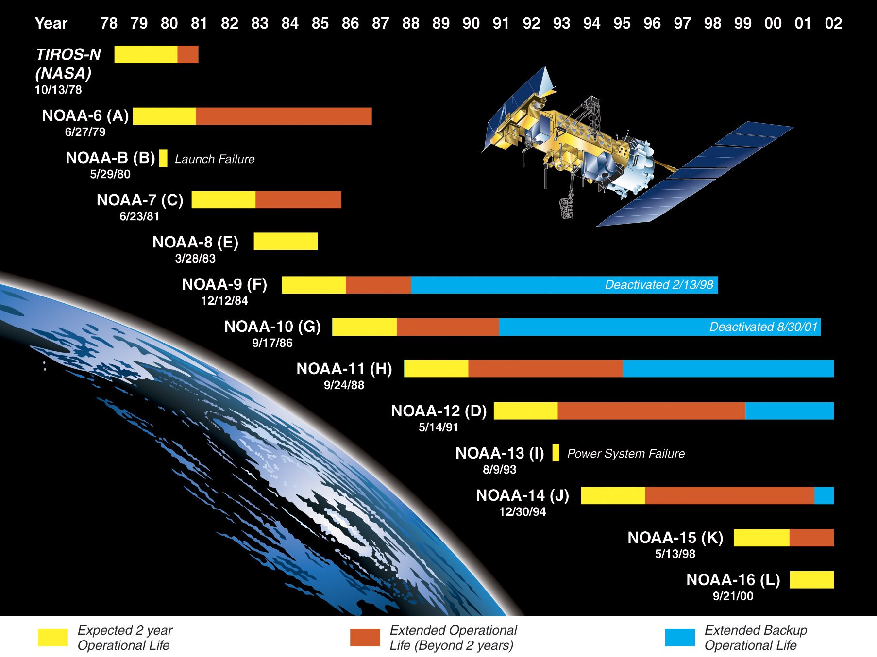
The first operational eyes were modest. A single-satellite temperature sounder had flown as early as Nimbus-3 in April 1969, and within a year its data had been coaxed into the National Meteorological Center’s analyses – the first satellite-sounding assimilation.⁶ But the first operational thermodynamic sounder on a routine weather satellite was the Vertical Temperature Profile Radiometer, an eight-channel infrared instrument on NOAA-2 through NOAA-5, producing routine soundings from November 1972 to February 1979.⁹ NOAA-2, the first to carry it, launched on 15 October 1972.⁹ The VTPR was an infrared filter radiometer sounding the 15-micrometre carbon-dioxide band. The definitive early report on its retrievals came from a NOAA scientist named Lawrence McMillin – of whom much more shortly.¹⁰

The instrument that defined the sounding era arrived on TIROS-N, launched 13 October 1978 into a sun-synchronous orbit near 830 to 845 kilometres.¹¹ It carried the TIROS Operational Vertical Sounder, TOVS – three instruments that would fly, in essentially the same form, on every operational NOAA polar orbiter from TIROS-N through NOAA-14, supplying the world’s temperature soundings for more than twenty years. They split the work. The High Resolution Infrared Radiation Sounder, HIRS/2, had twenty channels – nineteen infrared, one visible – across the carbon-dioxide bands for tropospheric and lower-stratospheric temperature, the water-vapour bands for humidity, an ozone channel and window channels, sampling at about 40 kilometres. The Microwave Sounding Unit, MSU, had four channels in the oxygen complex near 50 to 58 gigahertz, giving temperature at coarser resolution but with a property the infrared lacked. The Stratospheric Sounding Unit, SSU, had three channels near 15 micrometres, using pressure-modulated carbon-dioxide cells to reach up into the upper stratosphere.¹²

TOVS was limited by resolution. Individual infrared weighting functions were five to ten kilometres deep, and even by combining overlapping channels the effective vertical resolution of the retrieved profile was only about three kilometres – coarse against a radiosonde, which resolves features a few hundred metres thick.⁶ A sounder does not see the atmosphere in sharp layers. It sees it through broad, overlapping, smeared windows. That broadness and overlap is exactly what made the next step – turning radiances into temperature profiles – a genuinely hard problem, and it is where the retrieval era hit its ceiling.

4. The retrieval era and its ceiling

The instinctive way to use a satellite sounder is to make its data look like data you already know how to handle. The analysis systems of the 1970s and 1980s were built for radiosondes – vertical profiles of temperature and humidity at fixed levels. So the obvious move was to invert the measured radiances into a temperature profile, a “retrieval,” and feed that profile into the analysis as though it were a radiosonde launched from a balloon that happened to be a satellite. Retrieve, then assimilate. For fifteen years every major centre used the satellite soundings this way.

The trouble is that the inversion is ill-posed. Recovering a continuous temperature profile from a handful of broad, overlapping weighting functions is like reconstructing the exact shape of a bell from the single note it rings. Many different profiles produce almost the same radiances, so the solution is neither unique nor stable – a tiny change in the measured radiances, or in the instrument’s calibration, swings the retrieved profile wildly. To get any answer at all you must add information from outside the measurement: a prior, a first guess, to regularise the retrieval against. In the statistical-regression retrievals of the era that prior was usually a climatological mean profile, or regression coefficients trained on historical radiosonde-and-radiance pairs.⁶

The pioneer of the operational retrieval, and of the radiative-transfer corrections it needed, was Lawrence McMillin at NOAA’s National Environmental Satellite Service in Camp Springs, Maryland. Central to the sounding programme from the VTPR onward, McMillin devised one of the most elegant ideas in the enterprise: the split-window technique. Even a “window” channel chosen to see the surface is contaminated by water vapour in the intervening air, so the brightness temperature it reports is not quite the surface temperature. McMillin’s fix, worked out in the mid-1970s and validated in his 1984 paper with D. S. Crosby, was to use two nearby window channels whose water-vapour absorption differs slightly. The atmospheric contamination differs between the two channels but the surface signal is the same, so the difference between their brightness temperatures measures the atmospheric correction directly – subtract it out, and the true surface temperature falls out. It is the archetype of a family of techniques that use channel differences to cancel an unknown, and it made operational satellite sea-surface temperature possible.¹³

But the split window, ingenious as it is, is as much a symptom of the deeper difficulty as a cure for part of it. The retrieve-then-assimilate paradigm had a flaw no cleverness at the retrieval stage could fix, and it took a careful error analysis to expose. John Eyre, whose work is the hinge of this story, later laid it out. Write the retrieval as a linear estimate: retrieved profile equals first guess, plus a gain matrix times the gap between the measured radiances and the radiances the first guess would produce. Push the errors through and the error in the retrieved profile splits in two. One part is the measurement error in the radiances – expected, benign, roughly uncorrelated from one sounding to the next. The other is the error in the first guess, and that part is the poison. When the first guess is a climatological mean, neighbouring soundings all share essentially the same first-guess error, so the retrievals inherit errors correlated across space and, worse, correlated with the synoptic situation itself.⁶

Correlated observation error is an analysis system’s nightmare, because the standard analysis assumes the opposite. Optimum interpolation and its variational descendants treat observation errors as independent, so a crowd of nearby observations beats the analysis error down as it grows. Feed them a field of soundings whose errors are all correlated – all biased the same way by the same shared climatological background in the same weather regime – and the system thinks it has many independent measurements confirming one another when it really has one systematic error, repeated. It marches the analysis confidently toward a wrong answer. Erik Andersson and colleagues at ECMWF documented exactly these synoptically correlated biases in the TOVS layer-mean temperatures in 1991.¹⁴

The result was a slow crisis of confidence through the late 1980s. As short-range forecasts improved – as the first guess got better – the marginal value of the coarse, correlated-error TOVS retrievals shrank, and in the well-observed North it turned negative. At ECMWF the impact of TOVS retrievals on Northern-Hemisphere skill went from clearly positive in the early 1980s, to neutral, to actively harmful by the late 1980s. The analysis was better without the satellite soundings than with them.⁶ Graeme Kelly and Jean Pailleux tried to rescue it by coarsening the retrievals, keeping only the broad layers TOVS could genuinely resolve – from fourteen thickness layers in the early 1980s down to eleven, then seven. That held the Southern-Hemisphere impact positive but never made the Northern impact reliably good.⁶ The retrieval paradigm had hit its ceiling. The satellites were flying, the radiances were pouring in, and the best method anyone had was making the Northern forecast worse. The way out was not a better retrieval. It was to stop retrieving.

5. The turn: putting the physics inside the analysis

The move that broke the ceiling needs no symbols. Say you want the atmosphere’s temperature profile, and your instrument reports not temperature but a set of brightness temperatures – loosely, the “colours” of the infrared and microwave light leaving the top of the atmosphere. Two ways to proceed. Work backwards: invert the colours into a profile and hand it to the analysis. That is retrieval, and we have just seen why it fails – the inversion is ill-posed and smuggles correlated first-guess error into the analysis. Or turn the problem around. Keep a physics model that predicts, for any candidate temperature profile, what colours the satellite ought to see. Then invert nothing. Search among possible states of the atmosphere for the one whose predicted colours best match the measured colours, while staying close to the short-range forecast. Run the physics forwards, compare simulated with measured radiances, adjust the state until they agree. No inversion ever happens; the ill-posedness is handled quietly and optimally by the forecast constraint already built into the analysis. This is direct radiance assimilation.

Its natural home is the variational analysis. Recall from Post 47 that a variational assimilation defines a cost function measuring how badly a candidate atmospheric state misfits two things at once – the background forecast and the observations – then finds the state that minimises it.³ The observation part carries an observation operator, written $H$, which maps the atmospheric state into the quantity the instrument measures, so simulated and observed values can be compared in the instrument’s own terms. For a radiosonde temperature, $H$ is almost trivial: interpolate the model temperature to the balloon. The whole leap of direct radiance assimilation is to make $H$ a radiative-transfer model – a physics calculation that takes a model profile of temperature and humidity and returns the brightness temperatures a given channel would measure. The cost function then reads, in the form John Eyre used in his own review:

\[J(\mathbf{x}) = \tfrac{1}{2}(\mathbf{x} - \mathbf{x}_b)^\top \mathbf{B}^{-1} (\mathbf{x} - \mathbf{x}_b) + \tfrac{1}{2}\big(\mathbf{y} - H[\mathbf{x}]\big)^\top (\mathbf{E} + \mathbf{F})^{-1} \big(\mathbf{y} - H[\mathbf{x}]\big).\]

Here $\mathbf{x}$ is the atmospheric state being solved for – the profiles of temperature, humidity and the rest; $\mathbf{x}_b$ is the background, the short-range forecast first guess; $\mathbf{B}$ is the covariance of the background error, encoding how much the first guess can be trusted and how its errors are structured; $\mathbf{y}$ is the observation vector, which in direct radiance assimilation is the set of measured brightness temperatures; $H[\mathbf{x}]$ is the observation operator – the radiative-transfer forward model – which turns a model atmospheric state into the radiances the satellite should see; and $\mathbf{E}$ and $\mathbf{F}$ are the error covariances of the measurement and of the forward model respectively.⁶ In words: the analysis is the atmospheric state that at once stays close to the forecast (first term, weighted by trust in the forecast) and reproduces the radiances the satellite actually measured (second term, weighted by trust in the instrument and its forward model). Because $H$ is the radiative-transfer physics itself, and the background term keeps the problem well-posed, no ill-posed inversion appears anywhere. And there is a gift the retrieval approach could never give: when the model’s simulated radiances already match the measured ones, the second term contributes nothing, the analysis increment is zero, and the scheme invents no structure the data do not support.⁶

Two features of the variational framework made it the only practical vehicle, and John Eyre named both. First, nonlinearity. The radiative-transfer operator is nonlinear – Planck’s law and the exponential attenuation of radiation through the atmosphere are not linear in temperature – and optimum interpolation, the analysis method of the previous era described in Post 44 of this series, was built on linear estimation theory and could not easily swallow it.¹⁵ A variational cost function, minimised iteratively, handles nonlinearity without complaint. Second, dimensionality. Optimum interpolation, in the form Andrew Lorenc brought to ECMWF in 1981, requires inverting a matrix whose size scales with the number of observations – hopeless when the observations are millions of radiances.¹⁵ The variational method never forms that matrix. It minimises the cost function by following its gradient, and each step scales gently with the number of observations. So variational assimilation and direct radiance assimilation were, as Eyre put it, two faces of one event. Direct radiance assimilation was the variational engine’s first great customer, and radiances were why the engine had to scale to millions of observations.⁶¹⁴

The bridge from the retrieval era to full direct radiance assimilation was built by John Eyre himself, at ECMWF and the Met Office, and it was called one-dimensional variational analysis, 1D-Var. Apply the variational cost function above at a single sounding location, using only the vertical, with the short-range forecast profile and its error covariance as the constraint in place of a climatological prior. Eyre set out the theory in a two-part 1989 paper, “Inversion of cloudy satellite sounding radiances by nonlinear optimal estimation.”¹⁶ The scheme went operational on TOVS at ECMWF in June 1992, documented by Eyre with Kelly, Anthony McNally, Erik Andersson and Anders Persson in 1993.¹⁷ In that early hybrid, 1D-Var sat between the raw radiances and the still-operational optimum-interpolation analysis: it used the forecast as background to turn radiances into a forecast-consistent retrieval, free of the climatological pathology, that the interpolation analysis could safely ingest. It was retrieval done right – retrieval against the forecast, not against climatology – and it stood one variational step from dropping the retrieval altogether.

None of this was operationally possible without software, and here the “machine” driving the revolution is code, not hardware. A variational analysis evaluates the observation operator $H$, and its derivatives, for every radiance at every iteration of the minimisation – millions of radiative-transfer calculations per cycle, all of which must finish inside a fixed operational window measured in minutes. A full line-by-line computation, summing absorption over thousands of spectral lines, is far too slow. The answer was the fast radiative-transfer model, and at ECMWF and the Met Office it took the form of RTTOV, originally “Radiative Transfer for TOVS.” RTTOV swaps the line-by-line sum for fast regression: the layer optical depths that govern transmission are approximated as polynomials in a few profile variables, with the coefficients trained in advance against accurate line-by-line models. Trade a little accuracy for orders of magnitude of speed – and that trade is what makes operational radiance assimilation possible.¹⁸ Because $H$ now lives inside a gradient-based minimisation, RTTOV had to supply not only the forward calculation but its tangent-linear, adjoint and Jacobian versions – the derivatives that tell the minimisation how each brightness temperature responds to a change in temperature or humidity at each level. The model had to be differentiable, not just fast.⁶

RTTOV’s lineage runs from Eyre and Woolf’s fast-transmittance work of 1988, through the first version proper in Eyre’s 1991 ECMWF technical memorandum, through revisions by Rayer, by Rizzi and Matricardi, and by Roger Saunders and Matricardi in 1999.¹⁸ In the mid-1990s, when EUMETSAT set up its network of Satellite Application Facilities, the Numerical Weather Prediction facility – led by the Met Office – adopted RTTOV as a shared community package, and Roger Saunders, head of the Satellite Section at ECMWF from 1995 to 1999, became its long-time scientific lead. By the 2010s RTTOV had more than a thousand registered users worldwide, its version history set out by Saunders and colleagues in Geoscientific Model Development in 2018.¹⁹ The logic of the shared facility was institutional as much as scientific: as Eyre noted, no single centre could maintain expertise on the observation operator for every satellite instrument, so the fast radiative-transfer model became common infrastructure rather than mere code, mirrored on the American side by the Joint Center for Satellite Data Assimilation and its Community Radiative Transfer Model.⁶

6. Operational adoption: the direct radiance era begins

The paper that carried direct radiance use into the variational framework was Erik Andersson, Jean Pailleux, Jean-Noël Thépaut, John Eyre, Anthony McNally, Graeme Kelly and Philippe Courtier, “Use of cloud-cleared radiances in three/four-dimensional variational data assimilation,” 1994.²⁰ The author list repays a second look. It is the ECMWF satellite-and-assimilation group of the mid-1990s, in one place. Thépaut and Courtier – readers of Post 47 will know Courtier as the man who put four-dimensional variational assimilation on the operational schedule – were at the same time building the four-dimensional engine that Post 47 is about. Anthony Hollingsworth, absent from this paper but presiding over the programme as Head of Research, was the Irish-born patron of the whole variational effort; Post 47 readers will know him too.³ The satellite side and the variational-engine side of ECMWF were, in the mid-1990s, the same small group of people.

The qualifier in the title – cloud-cleared – marks a compromise of the period, and shows how much early direct-radiance work was still shadowed by the infrared’s blindness to cloud. An infrared channel over a cloudy scene reports the temperature of the cloud top, not of the column, so the early variational schemes could not simply take every infrared radiance as it arrived. Instead they ran a cloud-clearing step, combining several adjacent fields of view to estimate what the radiance would have been with no cloud, and assimilated that. Cloud-clearing recovered some information from partly-cloudy scenes, threw away the overcast ones, and added error of its own. The deeper fix came later, from two directions: the microwave sounders, which saw through cloud to begin with, and, later still, all-sky schemes that modelled the cloud and precipitation inside the radiative transfer instead of clearing them away. But in the mid-1990s cloud-cleared infrared radiances alongside the emerging microwave radiances were the state of the art, and they were enough to start narrowing the gap.²⁰⁶

The first operational deployment came not in Europe but in the United States. The National Centers for Environmental Prediction had put the world’s first operational three-dimensional variational analysis – the Spectral Statistical Interpolation, SSI – into service in June 1991, closing the optimum-interpolation loop traced in Post 44.¹⁵²¹ Into that framework John Derber and colleagues added direct clear-sky assimilation of infrared and microwave radiances in the mid-1990s, so the American analysis was ingesting raw radiances before the European one.²¹ ECMWF followed on 30 January 1996, when its three-dimensional variational analysis went operational assimilating cloud-cleared TOVS radiances directly, retiring nearly two decades of optimum interpolation.²² Twenty-two months later, on 25 November 1997, ECMWF switched to four-dimensional variational assimilation, and direct radiance assimilation entered the four-dimensional era – the deployment Post 47 is built around.³¹⁴ ECMWF’s own retrospective is blunt about the pair: “the transition to variational assimilation and direct radiance assimilation resulted in the largest changes to operational forecast scores at the end of the 1990s.”¹⁴

The other centres joined over the following decade, each on its own schedule. The Met Office, home to Eyre and Saunders, moved to variational assimilation of radiances around 1999 and to four-dimensional variational assimilation in 2004.⁶ The Japan Meteorological Agency began operational direct assimilation of ATOVS radiances in its global three-dimensional variational system on 28 May 2003.²³ But the calendar of deployments is not the point. The point is that direct radiance assimilation and variational assimilation had fused into a single operational paradigm, and the satellites were at last being used in a way that did not spoil the well-observed hemisphere. The observing system was now set for its largest single leap. That leap was made of microwaves.

7. The AMSU leap

The infrared has a fatal blindness, and it explains why the retrieval-era gains had clustered over the clear-sky Southern oceans instead of the stormy regions where forecasts matter most. Cloud droplets run a few micrometres to some tens of micrometres across, comparable to infrared wavelengths, so cloud strongly absorbs and scatters infrared radiation. An infrared sounder over a cloud deck sees the cloud top and nothing under it; the temperature structure below is hidden. But the meteorologically active regions – fronts, developing cyclones, the systems the forecast most needs to capture – are the cloudy ones. The infrared sounds best where the weather is quietest.⁶

Microwaves solve it. A microwave wavelength of a few millimetres is far larger than a cloud droplet, so non-precipitating cloud is nearly transparent to it: the microwave sounder reads the temperature of the air through the cloud, in exactly the disturbed, cloud-covered regions where the infrared goes blind. TOVS had carried a microwave temperature sounder from the start – the four-channel MSU – but four channels give only a coarse profile, and the instrument could do little more. The change came when the microwave sounder was rebuilt at far higher spectral resolution.

The cross-track scan geometry of a microwave sounder of the AMSU family: the instrument sweeps a mirror from side to side across the sub-satellite track while the spacecraft's forward motion advances the swath, tiling the surface beneath the orbit with sounding footprints. Unlike the infrared, these microwave soundings are made almost regardless of cloud. Diagram: Peteymills (English Wikipedia), public domain.

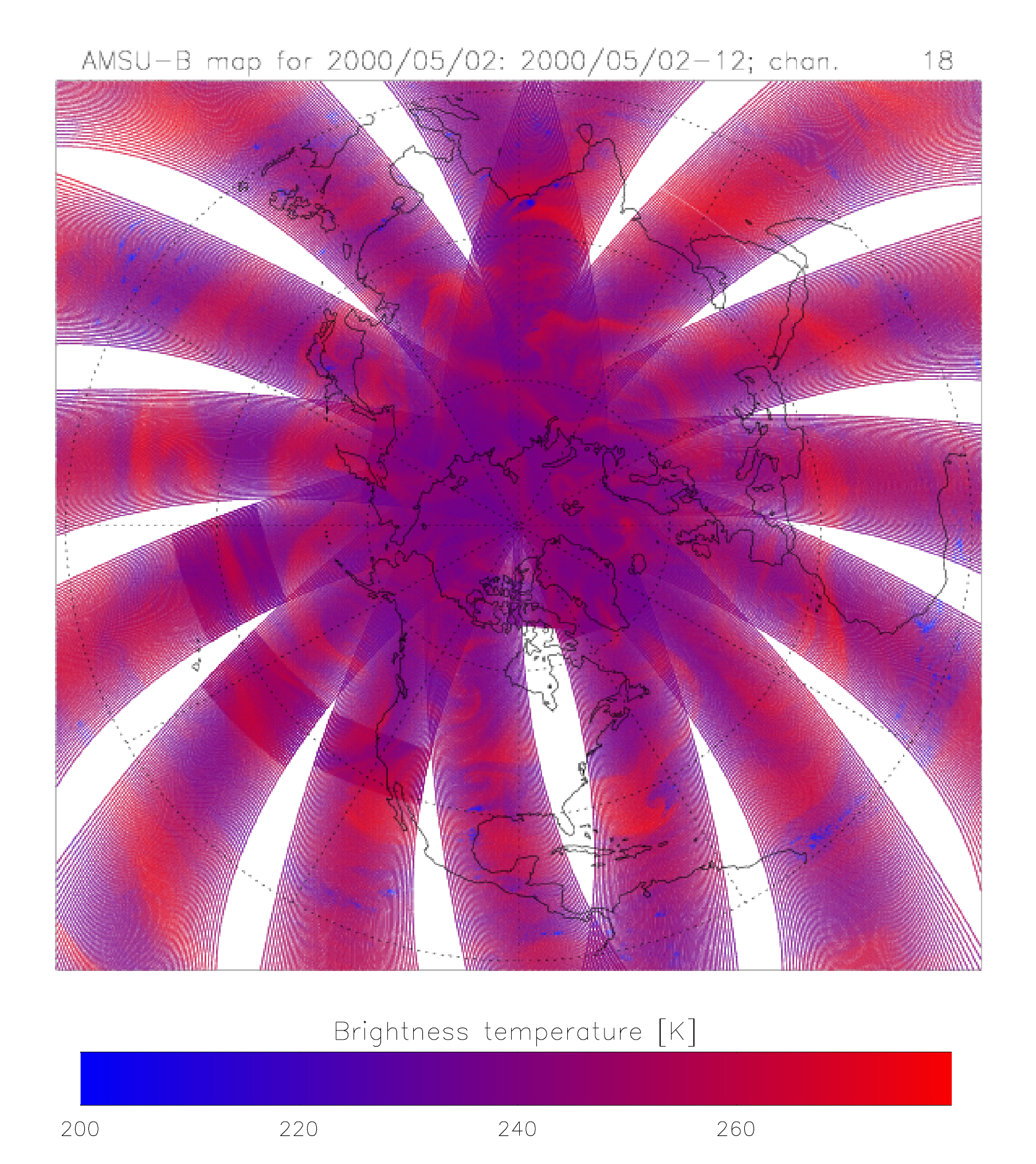
That rebuilt instrument was the Advanced Microwave Sounding Unit, and it first flew on NOAA-15, launched 13 May 1998 – the start of the ATOVS era, the “Advanced” TOVS.²⁴²⁵ AMSU came in two parts. AMSU-A had fifteen channels between 23.8 and 89 gigahertz, most arrayed across the oxygen complex to give a temperature profile from the surface up into the stratosphere, at far finer vertical resolution than the four-channel MSU it replaced – and, the decisive property, through cloud.²⁵ AMSU-B had five channels between 89 and 183.3 gigahertz for humidity.²⁵ With a third-generation infrared HIRS, the two AMSU instruments made up ATOVS. ATOVS radiances went operational at ECMWF in May 1999, and the effect on the Southern Hemisphere was immediate and large.⁶

Why did the South gain more than the North? It comes down to what each already had. The North had its dense radiosonde and aircraft network feeding temperature into the disturbed regions, so an all-weather microwave sounder there added real but incremental value. The South had almost nothing in those regions, and now suddenly had a temperature profile through the heart of every cloud-covered cyclone in the Southern Ocean, taken four times a day by the polar orbiters. Eyre’s own verdict on AMSU was that it “provided sounding quality in cloudy areas that had only been available hitherto in cloud-free areas,” and that this was “crucial to the performance of NWP systems.”⁶ The all-weather microwave temperature sounder did more than any other single instrument to lift the Southern skill curve toward the Northern. And the timing is no accident: the convergence Simmons and Hollingsworth documented – the South’s one-day gain compressed into about three years – falls in exactly the window when direct variational assimilation (1996-97) and the AMSU leap (1998-99) arrived together.¹ Engine and instrument reinforced each other. The microwave radiances were the new information; direct variational assimilation was the only method that could use them without the correlated-error pathology that had crippled the retrieval era.

The microwave family kept growing. AMSU-B gave way to the Microwave Humidity Sounder on later spacecraft; the Special Sensor Microwave/Imager on the American defence satellites, flying since 1987, supplied microwave imagery of surface wind, water vapour and cloud liquid over the data-sparse oceans.²⁶ In 2011 the Advanced Technology Microwave Sounder, a single twenty-two-channel instrument folding together the temperature and humidity heritage of AMSU-A and AMSU-B, flew on the Suomi National Polar-orbiting Partnership spacecraft, launched 28 October 2011.²⁷²⁸ But the principle that mattered was already fixed by AMSU-A in 1998: a temperature profile through cloud, made globally, four times a day. When the forecast-sensitivity experiments of the 2000s ranked the whole observing system by its contribution to skill, this instrument sat at the top.

8. The hyperspectral flood

If the microwave leap was about seeing through cloud, the next step was about spectral resolution – seeing the atmosphere in thousands of colours instead of tens. The TOVS infrared sounder, HIRS, had nineteen infrared channels, each a broad slice of spectrum admitted through a filter. A broad channel averages the emission over a wide band, and because broad channels’ weighting functions overlap heavily, nineteen of them resolve the vertical temperature structure only into layers a few kilometres thick. Sharpen it by narrowing the channels: a spectrally narrow channel placed on the flank of a single absorption line has a sharper, more localised weighting function, and a dense comb of such channels across a band builds a finely-spaced staircase that resolves thinner layers. This is the hyperspectral infrared sounder.

The NASA Aqua satellite, launched 4 May 2002, which carried the Atmospheric Infrared Sounder, AIRS -- the first hyperspectral infrared sounder to be exploited operationally in numerical weather prediction, with 2378 channels where TOVS had nineteen. Illustration: Reto Stoeckli, NASA Earth Observatory, 2009, public domain.

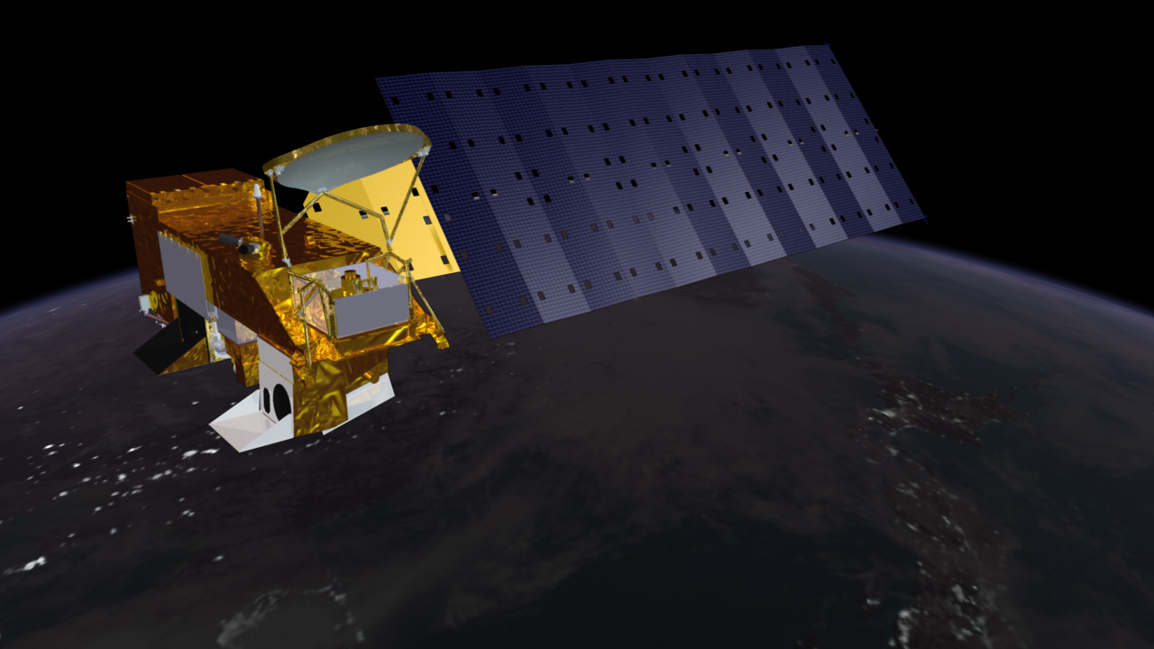
The first exploited operationally was the Atmospheric Infrared Sounder, AIRS, launched aboard NASA’s Aqua satellite on 4 May 2002. AIRS was a grating spectrometer with 2378 infrared channels spanning 3.7 to 15.4 micrometres – about a hundred times the spectral resolution of the old HIRS.²⁹ It flew as a research instrument, but the forecasting centres seized on it, and ECMWF was assimilating its radiances within a couple of years. Four years on came a still more capable instrument on the European side: the Infrared Atmospheric Sounding Interferometer, IASI, launched aboard MetOp-A on 19 October 2006. IASI was neither a filter radiometer nor a grating spectrometer but a Fourier-transform interferometer – a Michelson interferometer that recovers the full spectrum from an interferogram – yielding 8461 spectral samples across 645 to 2760 wavenumbers, about 15.5 down to 3.62 micrometres.³⁰ Where HIRS had resolved the temperature profile into layers about three kilometres thick, the hyperspectral sounders reached toward one.⁶

A European MetOp-class polar-orbiting meteorological satellite, of the line that has carried the IASI hyperspectral interferometer since MetOp-A in 2006. (The render is of the Second Generation platform; it stands here for the European polar-sounding line generally rather than for MetOp-A itself.) Illustration: ESA / ATG medialab, CC BY-SA 3.0 IGO.

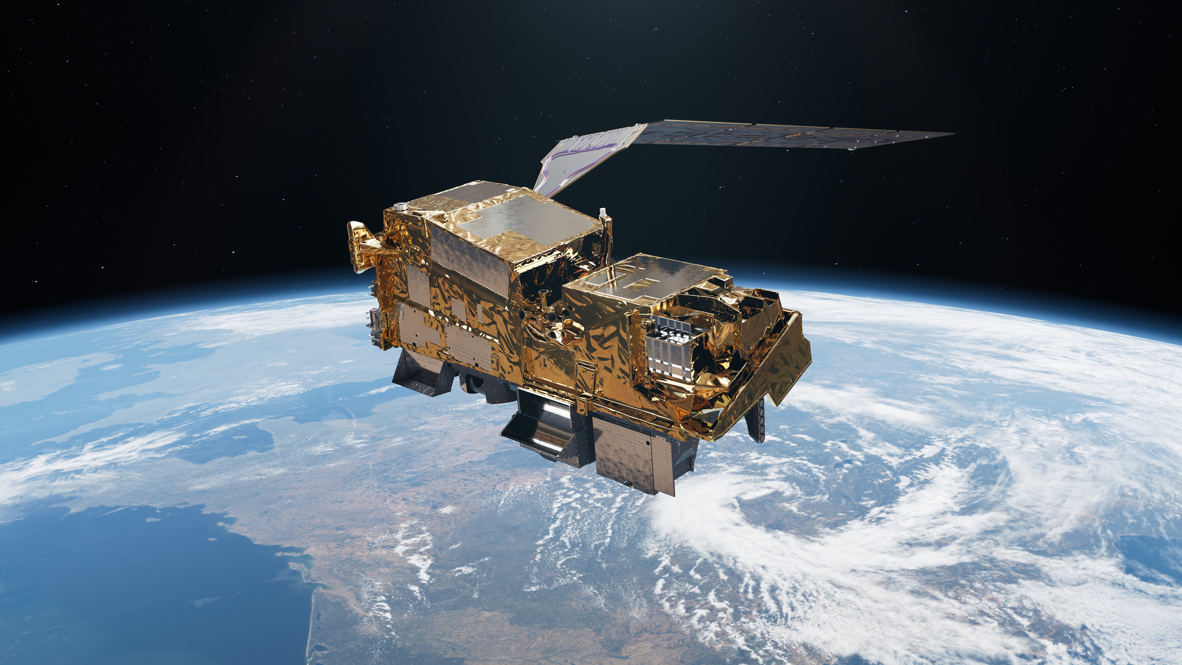
The two embodied two different technologies for slicing the infrared into thousands of pieces. AIRS dispersed the incoming infrared with a diffraction grating, much as a prism spreads white light, and read the resulting spectrum off an array of detectors, one per channel. IASI, built around a moving mirror, recorded not the spectrum but an interferogram – the signal made as the mirror sweeps and the two arms of the interferometer move in and out of phase – from which the full spectrum is recovered by a Fourier transform on the ground. The interferometer buys very high, very uniform spectral resolution across a wide band, at the price of that ground processing and of a subtlety called apodization: the deliberate smoothing of the instrument’s response to kill the ringing a sharp cutoff in the interferogram would otherwise produce. For the assimilation, the upshot was that IASI’s thousands of samples were narrow, uniform and finely spaced, ideal for building the staircase of weighting functions – but so numerous, and so correlated in their errors, that using them well demanded the channel-selection and error-modelling science that follows.³⁰⁶

But thousands of channels are not thousands of independent facts about the atmosphere, and reckoning with that is a branch of the science in itself. Many hyperspectral channels are redundant, their weighting functions nearly identical to their neighbours’; many are contaminated by cloud, by the surface, or by trace gases the analysis is not solving for; and no operational analysis can afford all 8461 of IASI’s samples every cycle. The channels have to be selected, and the framework for it is information-content theory, developed for atmospheric sounding by Clive Rodgers and applied to operational channel selection by, among others, Andrew Collard for IASI.³¹ The two standard measures are the degrees of freedom for signal – roughly, how many independent pieces of information the observations add beyond the background – and the Shannon information content, an entropy reduction. The sobering result: even a hyperspectral sounder with thousands of channels yields, for temperature and humidity together, an effective number of degrees of freedom only of order ten, because the weighting functions overlap so heavily.³¹ The vertical resolution sharpens to about a kilometre not because there are thousands of independent measurements but because thousands of overlapping narrow weighting functions are combined. The true information content is a modest handful of degrees of freedom, and knowing which channels carry it – which subset maximises the cumulative information while dodging cloud and surface contamination – is a real and continuing problem.³¹ The flood was real, but it was a flood you had to filter carefully to reach its modest, precious content.

9. A different kind of eye: radio occultation

Every observation so far – radiosonde, infrared radiance, microwave radiance – shares one weakness. Each rests on a calibration, and calibrations drift. A radiosonde’s temperature sensor carries a bias that depends on the manufacturer and on solar heating; a satellite radiometer’s calibration wanders as the instrument ages in orbit; the fast radiative-transfer model has its own systematic errors from imperfect spectroscopy. But one class of atmospheric observation is essentially self-calibrating, traceable not to a drifting sensor but to the most precise measurement we make – the measurement of time. It entered operational weather prediction in the 2000s as a different kind of eye.

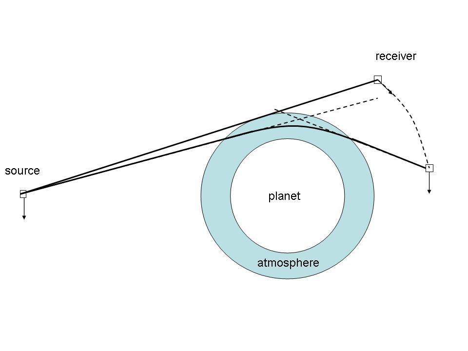
The technique is GPS radio occultation. A satellite in low Earth orbit watches a GPS satellite set behind the Earth’s limb. As the line of sight from receiver to transmitter sinks through ever denser air, the radio signal is bent by the vertical gradient of atmospheric density, and the deeper the ray, the more it bends. The receiver measures the GPS signal’s phase with extraordinary precision, because GPS runs on atomic clocks; from the accumulated phase it gets the frequency shift, from the frequency shift the bending angle, and from the profile of bending angle against ray height the profile of atmospheric refractivity.³² The mini-analogy: it is like reading the temperature and density of a swimming pool by watching how much a straight stick seems to bend at each depth as you lower it in – except the “stick” is a radio beam, the “bending” is clocked by an atomic standard, and nothing in the chain is calibrated against a physical thermometer.

The geometry of GPS radio occultation: a receiver in low Earth orbit tracks a GPS transmitter as the ray path between them sinks through the atmospheric limb. The ray bends by an amount set by the vertical gradient of density; the bending, measured through the precisely known GPS signal phase, yields a profile of atmospheric refractivity and hence of temperature and humidity. Diagram: MPRennie / Wikimedia Commons, CC BY-SA 3.0.

The atmosphere’s refractivity is captured in a compact formula. Refractivity $N$ – the refractive index’s departure from unity, times a million – is a sum of a few physical contributions:

\[N = \kappa_1 \frac{p}{T} + \kappa_2 \frac{e}{T^2} + \kappa_3 \frac{n_e}{f^2} + \kappa_4 W.\]

The first term, pressure $p$ over temperature $T$, is the dry-air density contribution; it dominates in the upper troposphere and stratosphere, where radio occultation therefore gives a clean temperature. The second, water-vapour partial pressure $e$ over the square of temperature, dominates in the lower troposphere, where the technique senses humidity. The third, electron density $n_e$ over the square of the signal frequency $f$, is the ionospheric contribution – and it drops out almost entirely when the two GPS frequencies near 1.575 and 1.227 gigahertz are combined, because it depends on frequency while the neutral-atmosphere terms do not. The fourth, from liquid water, is negligible at GPS frequencies.⁶³² The measurement resolves the vertical finely, half a kilometre to a kilometre. Its horizontal resolution is coarse, around two hundred kilometres along the ray, and its random error about a kelvin. But the property that matters most is the systematic error: below about 0.2 kelvin, and independent of any onboard calibration.⁶

The geometry explains both the strengths and the limits. Because the ray runs nearly horizontally at its lowest point, radio occultation is a limb sounder: it integrates along a long, nearly-tangential path, which buys exquisite vertical resolution – the ray height changes slowly as the profile is traced – but coarse horizontal resolution, smeared over a couple of hundred kilometres. That is the mirror image of the nadir-viewing radiometers, which see a compact footprint on the ground but resolve the vertical only coarsely. The two eyes complement each other: the radiometers give horizontal detail and broad vertical coverage, the occultations give sharp vertical structure and an absolute temperature reference in the upper troposphere and lower stratosphere. Another reason radio occultation counts for far more than its data volume suggests – it does not duplicate the radiances but supplies the vertical sharpness and the calibration anchor the radiances most lack.³²⁶

The technique was demonstrated first by the GPS/MET experiment aboard the MicroLab-1 satellite in 1995, and validated against conventional data by Christian Rocken and colleagues at the University Corporation for Atmospheric Research in 1997.³³ The single-satellite CHAMP mission then supplied a continuous stream of occultations from 2000, and in 2006 Sean Healy and Jean-Noël Thépaut at ECMWF showed that assimilating the CHAMP measurements – specifically the bending angle itself, through a bending-angle observation operator, rather than a derived temperature or refractivity – improved the forecast.³⁴ The mission that turned radio occultation from a promising demo into an operational data source was COSMIC, or FORMOSAT-3: six microsatellites launched together from Vandenberg on a single Minotaur rocket on 15 April 2006, the world’s first operational radio-occultation mission, a US-Taiwan partnership delivering some three thousand occultation profiles a day.³⁵ Its American champion was Richard Anthes, born in St. Louis on 9 March 1944 and President of UCAR from 1988 to 2012, who had taken up radio occultation in the early 1990s and driven both the GPS/MET proof of concept and the COSMIC constellation; the ECMWF assimilation was led by Sean Healy.³⁶³⁵

Radio occultation’s self-calibrating character gives it a role out of all proportion to its data volume, and to see why you have to face a subtle failure mode of direct radiance assimilation. It compares measured brightness temperatures with model-simulated ones – but both carry systematic biases. The instrument’s calibration drifts; the fast radiative-transfer model has spectroscopic errors; the biases depend on channel, scan angle and air mass, and are often larger than the atmospheric signal the analysis is trying to extract. Uncorrected, they corrupt the analysis. The fix, developed at ECMWF by Dick Dee, is variational bias correction, VarBC. Dee had come to ECMWF as a visiting scientist in 2003-04 specifically to build automatic bias correction for the reanalysis stream. His method models each channel’s bias as a small linear combination of predictors – a constant offset, the scan angle, air-mass predictors such as layer thicknesses – and estimates the coefficients inside the variational cost function, alongside the atmospheric state, by enlarging the control vector.³⁷³⁸ The correction then adapts on its own, continuously, as instruments drift and new sensors join, with no manual offline retuning. Dee set out the scheme in an ECMWF workshop paper in 2004; Thomas Auligné, Anthony McNally and Dee gave the definitive treatment in the Quarterly Journal in 2007; and VarBC went operational in the ECMWF forecasting system in September 2006.³⁷³⁹⁴⁰

But VarBC carries a hazard of its own. If every observation is bias-corrected against the model background, nothing pins the absolute reference, and the whole system can drift together toward a biased state – confidently self-consistent and collectively wrong. The analysis needs an anchor: a class of observation trusted enough to be assimilated without bias correction, holding the system to the real atmosphere. Radiosondes serve partly. The ideal anchor is GPS radio occultation, because its systematic error is below 0.2 kelvin and traceable to the frequency standard rather than to any drifting instrument. Radio occultation is assimilated without bias correction, and so it anchors the bias correction of everything else.⁶³² That is the deep reason a technique delivering a few thousand profiles a day – a trickle beside the millions of radiances – is prized so highly. It is the fixed point against which the whole flood of radiances is calibrated. The self-calibrating eye keeps the observing system honest.

10. The proof: which eye matters most

By the late 2000s the observing system had grown enormous and heterogeneous – radiosondes, aircraft, ships and buoys, surface stations, atmospheric motion vectors from geostationary imagery, scatterometer winds, GPS radio occultation, and above all the flood of infrared and microwave radiances from a fleet of polar orbiters. A pressing question followed. Of all of these, which observations were actually doing the work? Which earned their cost, and which could be lost with little harm? Answering it meant attributing a share of the forecast improvement to each observing system, and the tool that made that possible was itself a child of the variational, adjoint-based machinery of Post 47.

The tool is forecast sensitivity to observations, FSOI, and its adjoint-based form was introduced by Rolf Langland and Nancy Baker at the United States Naval Research Laboratory in Monterey in 2004.⁴¹ Run the adjoint of the assimilation-and-forecast system, and it computes – cheaply, and for every single observation at once – how much that observation cut, or added to, the short-range forecast error. Sum over an observing system and a season, and you have that system’s share of the total forecast-error reduction. Carla Cardinali brought the method into operational practice at ECMWF, setting it out in the Quarterly Journal in 2009 and running it routinely after.⁴²⁴³⁴⁴

A word on what the method measures, and what it does not. Forecast sensitivity to observations gauges each observation’s impact on a short-range forecast error – usually the twenty-four-hour forecast, in a dry-energy norm – because the computation leans on the adjoint of the assimilation and forecast system, a linearisation valid only over short ranges. It tells you how each observation improved the very next forecast, summed over the whole system, not medium-range skill directly. Its virtue is reach: one adjoint calculation delivers the impact of every one of the millions of observations at once, split by instrument, variable, region and level – something no run of data-denial experiments, each needing its own full rerun, could ever afford. So the two approaches complement each other. Data denial is expensive and reaches into the medium range; the forecast-sensitivity diagnostic is cheap and reaches only the short range. Where they agree, as they do on the primacy of the microwave sounders, the conclusion is about as firm as observational meteorology allows.⁴²⁴⁴

The result, reproduced across centres and years, was consistent and striking. In her 2013 ECMWF lecture notes, computing over data from June to October 2011, Cardinali gave the ranking in a passage that settles the question:

The largest contribution to decreasing the forecast error is provided by AMSU-A (~25%), IASI, AIRS, AIREP (aircraft data) and GPS-RO observations account for 10% of the total impact, respectively. TEMP and SYNOP surface pressure observations contribute by 5% followed by AMVs and HIRS (~4%), then by ASCAT and DRIBU (3%). All other observations contribute to less than 3%.⁴⁵

The all-weather microwave temperature sounder introduced on NOAA-15 in 1998 was, by this reckoning, the single most valuable observing system on Earth – responsible for about a quarter of the entire reduction in short-range forecast error, more than twice the share of any other instrument type, and more than the hyperspectral infrared sounders with all their extra channels.⁴⁵ The independent adjoint-sensitivity study Sangwon Joo, John Eyre and R. Marriott ran on the Met Office global system in 2013 reached the same qualitative conclusion, AMSU-A and IASI the leading satellite contributors.⁴¹ One caution. The ranking is by total contribution, where the satellites win partly on sheer volume; per individual report, a conventional in-situ observation – a single radiosonde, a single buoy pressure – carries more weight, and it is the vast number of radiances that puts the microwave sounders on top.⁴³ But the operational verdict is not in doubt. Tracked as a category, the microwave sounders held the largest share of the total forecast-error reduction of any part of the observing system, and rising – from about 26% to 33% in a single year as new sounders came online.⁵

The complementary proof is the data-denial experiment, and its numbers are the quantitative heart of the “hemisphere that caught up” story. In a systematic 2019 study of global observing-system experiments, ECMWF scientists withheld whole classes of observation and measured the damage. The result was starkly asymmetric. In the Southern Hemisphere extratropics the microwave radiances were the dominant system: withholding them degraded the three-day 500 hPa forecast error by 11%, with a statistically significant impact out to day nine, while conventional data, infrared sounders and radio occultation each cost only a few per cent. In the Northern extratropics the picture flipped – there the conventional network was dominant, costing 10% at day three against the microwave sounders’ 6%.⁴⁶ That asymmetry is the convergence story told in the negative. The North is carried by its dense in-situ network, the South by microwave satellite sounders. Take the satellites away and the South slides back toward the observation-starved regime of about 1980 – the same “catastrophic degradation in the southern hemisphere” the 2013 review described, a collapse of roughly the pre-convergence gap of about one forecast day.⁵¹ And the worth of a single instrument, once the full system is in place? Losing one AMSU-A costs about half a per cent in the forecast scores – small only because so many others remain to cover for it.⁵

11. The convergence revisited

Return to the chart we began with: two climbing curves, the North above and the South below, the gap of a full day of predictability that held through the 1980s and then closed across the late 1990s and early 2000s until the curves nearly met.¹² We can now say what closed it. Not new radiosonde networks in the Southern Ocean – those were never built. What closed it was the shift, over roughly a decade, from a way of using satellite radiances that made the well-observed hemisphere’s forecast worse to a way that carried the poorly-observed hemisphere almost to parity. The shift had three interlocking parts, and no one of them would have done alone.

First, the intellectual turn from retrieval to direct assimilation – from inverting radiances into pseudo-radiosonde profiles, with all the ill-posedness and correlated error that carried, to placing a radiative-transfer forward model inside the analysis as the observation operator and assimilating the raw brightness temperatures directly. Only the variational analysis made that turn possible; it could take the nonlinear observation operator and scale to millions of observations, so direct radiance assimilation and variational assimilation arrived together, one coupled advance.⁶¹⁴ Second, the software that made the turn tractable: the fast, differentiable radiative-transfer model, RTTOV and its kin, without which the observation operator could not have been evaluated the millions of times per cycle the minimisation demanded. The enabling machine of this revolution was code, not silicon.¹⁸¹⁹ Third, the observing system’s own great leap – the all-weather microwave temperature sounder AMSU-A of 1998, which for the first time gave a temperature profile through the cloud-covered cyclones of the Southern Ocean, backed by the hyperspectral infrared flood of AIRS and IASI and anchored by the self-calibrating eye of GPS radio occultation.²⁵³⁰³⁵

Be clear about what the satellites did and did not do, because the temptation is to credit them with everything. The most careful attribution, by Dick Dee and Sakari Uppala from a thirty-year comparison of reanalysis against operations, found that better observations account for only about a quarter of the total forecast improvement over the era; the other three-quarters came from better data assimilation and better models.⁵⁴⁷ The convergence was satellite-driven, not satellite-only. The satellites supplied the raw information the South had lacked; the variational assimilation was what let that information – noisier, more indirect, more error-correlated than a radiosonde – be used at all. They are one achievement seen from two sides, and pulling them apart is a category error. The instrument without the method made the Northern forecast worse in 1988. The method without the instrument had nothing to work with over the Southern Ocean.

The convergence reaches one further place, and there it closes a loop with an earlier post. The reanalyses – retrospective reconstructions of the atmosphere’s history, produced by running a modern assimilation system over decades of archived observations, the subject of Post 46 of this series and of Eugenia Kalnay’s work at the National Centers for Environmental Prediction – rest entirely on the machinery described here.⁴⁸ A reanalysis of the satellite era is only as good as its handling of satellite radiances, and handling radiances across decades of drifting, changing instruments is the problem variational bias correction was built to solve. No coincidence, then, that Dee built VarBC as a member of ECMWF’s reanalysis team, recruited because the reanalysis could not proceed without automatic, adaptive bias correction of the radiance record.⁴⁷³⁸ Direct radiance assimilation, the fast radiative-transfer model, and the self-anchoring bias correction did more than close the forecast-skill gap in real time. They are what makes it possible to reconstruct the atmosphere’s past with a consistency the original observations, taken one drifting instrument at a time, could never have supplied on their own.

The Southern Hemisphere spent the first quarter-century of the satellite age as the poor relation of numerical weather prediction – a hemisphere whose forecasts, by the hard measure of the anomaly correlation, ran a full day behind. By the mid-2000s that was no longer true, and it has not been true since. A five-day forecast of the circulation over the Southern Ocean is now nearly as trustworthy as one over Europe. The reason is that the radiation measured by a fleet of polar-orbiting instruments – infrared and microwave brightness temperatures, and the bending of GPS signals through the limb – is now read straight into the analysis by a physics model of how photons leave the atmosphere, weighted against a forecast, corrected for its own biases against an atomic-clock anchor, and minimised in a variational cost function four times a day. The hemisphere half-blind for the whole satellite era learned, in a single decade, to see. The two curves are indistinguishable now, where for a quarter-century they had stood a full forecast day apart.

---

1. Simmons, A. J., and A. Hollingsworth, 2002: “Some aspects of the improvement in skill of numerical weather prediction,” Quarterly Journal of the Royal Meteorological Society 128(580), 647-677, DOI 10.1256/003590002321042135, https://rmets.onlinelibrary.wiley.com/doi/10.1256/003590002321042135. The full text is paywalled; the two quoted lines were read verbatim from the identical ECMWF Technical Memorandum 342 at https://www.ecmwf.int/sites/default/files/elibrary/2001/12238-some-aspects-improvement-skill-numerical-weather-prediction.pdf. This is the same verification paper that anchored Post 47; it documents the roughly one-day Southern-Hemisphere gain compressed into about three years and the “almost as skilful as those for the northern hemisphere” conclusion. ↩ ↩² ↩³ ↩⁴ ↩⁵ ↩⁶

2. Bauer, P., A. Thorpe and G. Brunet, 2015: “The quiet revolution of numerical weather prediction,” Nature 525, 47-55, 3 September 2015, DOI 10.1038/nature14956, https://www.nature.com/articles/nature14956. The opening figure, reproducing the converging Northern- and Southern-Hemisphere anomaly-correlation curves, became the canonical visual summary of the era. ↩ ↩² ↩³

3. See Post 47, “Eleven Years from the Adjoint”, on the operational deployment of four-dimensional variational assimilation at ECMWF on 25 November 1997, and on Philippe Courtier, Jean-Noël Thépaut, Florence Rabier and Anthony Hollingsworth – the variational engine of which direct radiance assimilation was the first great customer. ↩ ↩² ↩³ ↩⁴

4. ECMWF, “Quality of our forecasts,” at https://www.ecmwf.int/en/forecasts/quality-our-forecasts. The centre’s headline verification score is the lead time at which the high-resolution forecast’s 500 hPa geopotential anomaly correlation falls through 80%, a lead time now nearly equal in the two hemispheres. ↩

5. English, S., T. McNally, N. Bormann and colleagues, 2013: “Impact of satellite data,” ECMWF Technical Memorandum 711, October 2013, at https://www.ecmwf.int/sites/default/files/elibrary/2013/9301-impact-satellite-data.pdf. Source for the “narrowed dramatically” narrative of the post-2000 gap, the “catastrophic degradation in the southern hemisphere” quotation (citing Radnoti et al. 2009), the ~0.5% cost of denying a single AMSU-A, the 26% to 33% rise in the microwave-sounder share of forecast-error reduction, and the Dee and Uppala one-quarter/three-quarters attribution. ↩ ↩² ↩³ ↩⁴ ↩⁵

6. Eyre, J. R., 2007: “Progress achieved on assimilation of satellite data in numerical weather prediction over the last 30 years,” ECMWF Seminar on Recent Developments in the Use of Satellite Observations in NWP, 3-7 September 2007, at https://www.ecmwf.int/sites/default/files/elibrary/2008/9341-progress-achieved-assimilation-satellite-data-numerical-weather-prediction-over-last-30-years.pdf. Eyre’s first-person review is the richest single narrative source for the retrieval-to-direct-radiance arc: the weighting-function physics, the microwave-through-cloud argument, the retrieval-error analysis, the ATOVS May 1999 operational date, the AMSU “sounding quality in cloudy areas” quotation, the Gilchrist 1982 FGGE data-denial figures, and the accessible cost-function form all come from it. ↩ ↩² ↩³ ↩⁴ ↩⁵ ↩⁶ ↩⁷ ↩⁸ ↩⁹ ↩¹⁰ ↩¹¹ ↩¹² ↩¹³ ↩¹⁴ ↩¹⁵ ↩¹⁶ ↩¹⁷ ↩¹⁸ ↩¹⁹ ↩²⁰ ↩²¹ ↩²² ↩²³ ↩²⁴ ↩²⁵ ↩²⁶ ↩²⁷ ↩²⁸ ↩²⁹

7. See Post 41, “The Coyote Who Found Chaos”, on Edward Lorenz’s 1963 discovery of sensitive dependence on initial conditions and the predictability limit it set for weather forecasting – the reason a data-starved region loses forecast skill fastest. ↩

8. eoPortal, “Satellite inputs to Numerical Weather Prediction (NWP),” at https://www.eoportal.org/other-space-activities/nwp, on the polar-orbiting sounder constellation and its global-coverage role in the observing system. ↩

9. NOAA National Centers for Environmental Information, “Vertical Temperature Profile Radiometer (VTPR),” at https://www.ncei.noaa.gov/products/vertical-temperature-profile-radiometer. The VTPR was an operational eight-channel infrared sounder flown on NOAA-2 through NOAA-5, producing routine soundings from November 1972 to February 1979; NOAA-2 (ITOS-D) launched 15 October 1972. ↩ ↩²

10. McMillin, L. M., and colleagues: “Satellite infrared soundings from NOAA spacecraft,” NOAA Technical Report NESS 65, at https://www.ncei.noaa.gov/sites/default/files/2021-08/noaa-tr-ness65-McMillin-VTPR.pdf. McMillin authored the definitive early VTPR retrieval report at NOAA’s National Environmental Satellite Service. ↩

11. “TIROS-N,” Wikipedia, https://en.wikipedia.org/wiki/TIROS-N. TIROS-N launched 13 October 1978 into a sun-synchronous orbit near 830-845 km and carried the TOVS suite. ↩

12. NOAA CLASS, “TOVS/ATOVS,” and the CEDA TOVS instrument record, at https://www.class.noaa.gov/release/data_available/tovs_atovs/index.htm. TOVS comprised HIRS/2 (20 channels: 19 infrared plus 1 visible), MSU (4 channels in the 50-58 GHz oxygen complex), and SSU (3 channels near 15 micrometres using pressure-modulated carbon-dioxide cells). ↩

13. McMillin, L. M., and D. S. Crosby, 1984: “Theory and validation of the multiple window sea surface temperature technique,” Journal of Geophysical Research: Oceans 89(C3), 3655-3661, DOI 10.1029/JC089iC03p03655, https://agupubs.onlinelibrary.wiley.com/doi/abs/10.1029/JC089iC03p03655. The split-window technique is usually traced to McMillin’s earlier work of the mid-1970s (commonly cited as McMillin 1975, JGR 80, 5113-5117), but that primary paper was not consulted during research and no hard year is asserted here; the confirmed primary is the 1984 validation paper. ↩

14. ECMWF, 2025: “Fifty years of data assimilation at ECMWF,” at https://www.ecmwf.int/sites/default/files/elibrary/81650-fifty-years-of-data-assimilation-at-ecmwf.pdf. Confirms the sequence Eyre 1989, Andersson et al. 1991 and 1994, Thépaut et al. 1996, 3D-Var 1996 and 4D-Var 1997, and the statement that “the transition to variational assimilation and direct radiance assimilation resulted in the largest changes to operational forecast scores at the end of the 1990s.” ↩ ↩² ↩³ ↩⁴ ↩⁵

15. See Post 44, “The Book That Crossed the Iron Curtain”, on Lev Gandin’s 1963 Leningrad monograph, the optimum-interpolation framework, and its transmission to the West through Andrew Lorenc at ECMWF – the linear, matrix-inverting analysis method that direct radiance assimilation could not have run on. ↩ ↩² ↩³

16. Eyre, J. R., 1989: “Inversion of cloudy satellite sounding radiances by nonlinear optimal estimation. I: Theory and simulation for TOVS,” Quarterly Journal of the Royal Meteorological Society 115(489), 1001-1026 (Part II, 1027-1037), https://rmets.onlinelibrary.wiley.com/doi/abs/10.1002/qj.49711548902. ↩

17. Eyre, J. R., G. A. Kelly, A. P. McNally, E. Andersson and A. Persson, 1993: “Assimilation of TOVS radiance information through one-dimensional variational analysis,” Quarterly Journal of the Royal Meteorological Society 119(514), 1427-1463, https://rmets.onlinelibrary.wiley.com/doi/abs/10.1002/qj.49711951411. One-dimensional variational analysis became operational on TOVS at ECMWF in June 1992. ↩

18. The RTTOV fast radiative-transfer model traces from Eyre and Woolf (1988) through Eyre (1991, ECMWF Technical Memorandum 176, the first RTTOV), Rayer (1995), Rizzi and Matricardi (1998), and Saunders, R., M. Matricardi and P. Brunel, 1999: “An improved fast radiative transfer model for assimilation of satellite radiance observations,” Quarterly Journal of the Royal Meteorological Society 125(556), 1407-1425 (ECMWF Technical Memorandum 282), at https://nwpsaf.eu/oldsite/deliverables/rtm/papers/tm282.pdf. RTTOV is now maintained through the EUMETSAT NWP SAF with Roger Saunders, head of the ECMWF Satellite Section 1995-1999, as long-time scientific lead. ↩ ↩² ↩³

19. Saunders, R., J. Hocking, E. Turner, P. Rayer, D. Rundle, P. Brunel, J. Vidot, P. Roquet, M. Matricardi, A. Geer, N. Bormann and C. Lupu, 2018: “An update on the RTTOV fast radiative transfer model (currently at version 12),” Geoscientific Model Development 11, 2717-2737, DOI 10.5194/gmd-11-2717-2018, https://gmd.copernicus.org/articles/11/2717/2018/. ↩ ↩²

20. Andersson, E., J. Pailleux, J.-N. Thépaut, J. R. Eyre, A. P. McNally, G. A. Kelly and P. Courtier, 1994: “Use of cloud-cleared radiances in three/four-dimensional variational data assimilation,” Quarterly Journal of the Royal Meteorological Society 120(517), 627-653, DOI 10.1002/qj.49712051707, https://rmets.onlinelibrary.wiley.com/doi/abs/10.1002/qj.49712051707. ↩ ↩²

21. NCEP/EMC data-assimilation history, at https://www.emc.ncep.noaa.gov/emc/pages/numerical_forecast_systems/ncep_data_assimilation.php. The Spectral Statistical Interpolation (SSI) three-dimensional variational analysis went operational in June 1991, and direct clear-sky infrared and microwave radiance assimilation was added to the global system in the mid-1990s (Derber and Wu 1998). ↩ ↩²

22. Courtier, P., E. Andersson, W. Heckley, J. Pailleux, D. Vasiljevic, M. Hamrud, A. Hollingsworth, F. Rabier and M. Fisher, 1998: “The ECMWF implementation of three-dimensional variational assimilation (3D-Var). I: Formulation,” Quarterly Journal of the Royal Meteorological Society 124(550), 1783-1807, https://rmets.onlinelibrary.wiley.com/doi/abs/10.1002/qj.49712455002. ECMWF 3D-Var with direct cloud-cleared TOVS radiances went operational on 30 January 1996 and ran to 24 November 1997. ↩

23. Kazumori, M., K. Okamoto and H. Owada, “Operational use of ATOVS radiances in global data assimilation at JMA,” RSMC Tokyo Technical Review No. 7, Numerical Prediction Division, Japan Meteorological Agency, at https://www.jma.go.jp/jma/jma-eng/jma-center/rsmc-hp-pub-eg/techrev/abs7.html. ATOVS radiances have been operationally assimilated in the JMA global three-dimensional variational system since 28 May 2003, replacing the TOVS/ATOVS retrievals used previously. ↩

24. ECMWF, 2018: “NOAA satellite launch 20 years ago marked start of new era,” on NOAA-15 (NOAA-K), launched 13 May 1998 as the first spacecraft to carry AMSU and to open the ATOVS era, at https://www.ecmwf.int/en/about/media-centre/news/2018/noaa-satellite-launch-20-years-ago-marked-start-new-era. ↩

25. “Advanced Microwave Sounding Unit,” Wikipedia, https://en.wikipedia.org/wiki/Advanced_microwave_sounding_unit. AMSU-A has 15 channels between 23.8 and 89 GHz (oxygen-band temperature sounding); AMSU-B has 5 channels between 89 and 183.3 GHz (moisture sounding). ↩ ↩² ↩³ ↩⁴

26. “Special sensor microwave/imager,” Wikipedia, https://en.wikipedia.org/wiki/Special_sensor_microwave/imager. The first SSM/I flew on the defence satellite DMSP F8 (launched 18 June 1987), a seven-channel dual-polarised microwave imager supplying surface wind, water vapour and cloud-liquid products over the oceans. ↩

27. “Advanced Technology Microwave Sounder,” Wikipedia, https://en.wikipedia.org/wiki/Advanced_Technology_Microwave_Sounder. ATMS is a 22-channel scanning microwave radiometer combining AMSU-A and AMSU-B/MHS heritage in a single instrument. ↩

28. “Suomi NPP,” Wikipedia, https://en.wikipedia.org/wiki/Suomi_NPP. Suomi NPP launched 28 October 2011 carrying the first ATMS. ↩

29. “Atmospheric Infrared Sounder,” Wikipedia, and the NASA JPL AIRS mission overview, at https://en.wikipedia.org/wiki/Atmospheric_infrared_sounder and https://www.jpl.nasa.gov/missions/atmospheric-infrared-sounder-airs/. AIRS launched on Aqua on 4 May 2002, a grating spectrometer with 2378 infrared channels spanning 3.7-15.4 micrometres. ↩

30. “Infrared Atmospheric Sounding Interferometer,” Wikipedia, https://en.wikipedia.org/wiki/Infrared_atmospheric_sounding_interferometer. IASI launched on MetOp-A on 19 October 2006, a Fourier-transform interferometer producing 8461 spectral samples across 645-2760 wavenumbers (15.5-3.62 micrometres). ↩ ↩² ↩³

31. Collard, A. D., 2011: “From observations to forecasts – Part 8: The use of satellite observations in numerical weather prediction,” Weather 66(2), https://rmets.onlinelibrary.wiley.com/doi/10.1002/wea.736. The information-content framework (degrees of freedom for signal, Shannon information content, averaging kernels) is that of Rodgers, C. D., 2000: Inverse Methods for Atmospheric Sounding: Theory and Practice, World Scientific; the effective degrees of freedom of order ten for a hyperspectral infrared sounder is illustrative rather than a hard instrument-specific figure. ↩ ↩² ↩³

32. Healy, S., 2008: “An introduction to GPS radio occultation and its use in numerical weather prediction,” ECMWF, at https://www.ecmwf.int/sites/default/files/elibrary/2008/9342-introduction-gps-radio-occultation-and-its-use-numerical-weather-prediction.pdf. Source for the refractivity relation, the two-frequency removal of the ionospheric term, the bending-angle operator, and the sub-0.2 K systematic error that makes radio occultation an unbiased anchor for variational bias correction. ↩ ↩² ↩³ ↩⁴

33. UCAR/COSMIC, “GNSS radio occultation,” at https://www.cosmic.ucar.edu/what-we-do/gnss-radio-occultation. GPS/MET aboard MicroLab-1 demonstrated radio occultation in 1995 (validated by Rocken et al. 1997); CHAMP provided occultations from 2000. ↩

34. Healy, S. B., and J.-N. Thépaut, 2006: “Assimilation experiments with CHAMP GPS radio occultation measurements,” Quarterly Journal of the Royal Meteorological Society 132(615), 605-623, DOI 10.1256/qj.04.182, https://rmets.onlinelibrary.wiley.com/doi/abs/10.1256/qj.04.182. Established the direct bending-angle observation operator for radio occultation at ECMWF. ↩

35. “FORMOSAT-3,” eoPortal, and the COSMIC/FORMOSAT-3 review in the Bulletin of the American Meteorological Society, 2020, at https://www.eoportal.org/satellite-missions/formosat-3 and https://journals.ametsoc.org/view/journals/bams/101/7/bamsD180290.xml. The six-satellite COSMIC/FORMOSAT-3 constellation launched from Vandenberg on a single Minotaur on 15 April 2006, the world’s first operational GPS radio-occultation mission, a US-Taiwan partnership delivering roughly 3000 occultation profiles a day. ↩ ↩² ↩³

36. “Richard A. Anthes,” Wikipedia, https://en.wikipedia.org/wiki/Richard_A._Anthes. Anthes was born 9 March 1944 in St. Louis, Missouri, and served as President of UCAR from 1988 to 2012, championing GPS/MET and COSMIC. ↩

37. Dee, D. P., 2004: “Variational bias correction of radiance data in the ECMWF system,” Proceedings of the ECMWF workshop on assimilation of high-spectral-resolution sounders in NWP, Reading, 28 June - 1 July 2004, at https://www.ecmwf.int/sites/default/files/elibrary/2004/8930-variational-bias-correction-radiance-data-ecmwf-system.pdf. ↩ ↩²

38. ECMWF, 2019: “Reanalysis pioneer Dick Dee bows out as ERA5 replaces ERA-Interim,” on Dee’s recruitment to the reanalysis team and his development of variational bias correction, at https://www.ecmwf.int/en/about/media-centre/news/2019/reanalysis-pioneer-dick-dee-bows-out-era5-replaces-era-interim. ↩ ↩²

39. Auligné, T., A. P. McNally and D. P. Dee, 2007: “Adaptive bias correction for satellite data in a numerical weather prediction system,” Quarterly Journal of the Royal Meteorological Society 133(624), 631-642, DOI 10.1002/qj.57, https://rmets.onlinelibrary.wiley.com/doi/abs/10.1002/qj.57. ↩

40. EUMETSAT NWP SAF and ECMWF, “Bias correction of satellite radiance observations at ECMWF,” confirming the operational implementation of variational bias correction in the ECMWF forecasting system in September 2006, at https://nwp-saf.eumetsat.int/site/download/ECMWF-VarBC.pdf. ↩

41. Langland, R. H., and N. L. Baker, 2004: “Estimation of observation impact using the NRL atmospheric variational data assimilation adjoint system,” Tellus A 56(3), 189-201; it introduced the adjoint-based observation-impact method used at the US Naval Research Laboratory on NOGAPS and NAVDAS, record at https://www.researchgate.net/publication/312359703. The Met Office corroboration is Joo, S., J. Eyre and R. Marriott, 2013: “The impact of MetOp and other satellite data within the Met Office global NWP system using an adjoint-based sensitivity method,” Monthly Weather Review 141(10), 3331-3342; that paper is paywalled and no per-instrument percentage is quoted here, only its qualitative finding that AMSU-A and IASI are the leading satellite contributors. ↩ ↩²

42. Cardinali, C., 2009: “Monitoring the observation impact on the short-range forecast,” Quarterly Journal of the Royal Meteorological Society 135(638), 239-250, DOI 10.1002/qj.366, https://rmets.onlinelibrary.wiley.com/doi/10.1002/qj.366. The original adjoint-based forecast-sensitivity-to-observations paper at ECMWF. ↩ ↩²

43. ECMWF, “Assessing the impact of observations using observation-minus-forecast residuals,” ECMWF Newsletter 152, at https://www.ecmwf.int/en/newsletter/152/meteorology/assessing-impact-observations-using-observation-minus-forecast. On the distinction between per-observation and per-observation-type impact: conventional in-situ reports carry the most weight per report, while satellites dominate the total by sheer volume. ↩ ↩²

44. ECMWF, 2009: “Forecast sensitivity to observations (FSO) as a diagnostic tool,” at https://www.ecmwf.int/sites/default/files/elibrary/2009/8578-forecast-sensitivity-observations-fso-diagnostic-tool-monitoring-impact-observations-short.pdf. ↩ ↩²

45. Cardinali, C., 2013: “Data assimilation: observation impact on the short range forecast,” ECMWF lecture notes, with the ranking computed over data from June to October 2011, at https://www.ecmwf.int/sites/default/files/elibrary/2013/16937-observation-impact-short-range-forecast.pdf. The ranked breakdown quoted in the text was read verbatim from this document; AMSU-A is the single most valuable observing system at about 25% of the total forecast-error reduction. ↩ ↩²

46. Bormann, N., and colleagues, 2019: “Global observing system experiments in the ECMWF assimilation system,” ECMWF Technical Memorandum 839, at https://www.ecmwf.int/sites/default/files/elibrary/2019/18859-global-observing-system-experiments-ecmwf-assimilation-system.pdf. Source for the data-denial numbers: in the Southern Hemisphere extratropics, withholding microwave radiances degrades the day-3 500 hPa error by 11%, significant to day 9; in the Northern Hemisphere extratropics, conventional data cost 10% and microwave 6% at day 3. ↩

47. Dee, D. P., and S. Uppala, 2009: “Variational bias correction of satellite radiance data in the ERA-Interim reanalysis,” Quarterly Journal of the Royal Meteorological Society 135(644), 1830-1841, DOI 10.1002/qj.493, https://onlinelibrary.wiley.com/doi/10.1002/qj.493. The one-quarter-observations / three-quarters-assimilation-and-model attribution over roughly thirty years is drawn from Dee and Uppala’s comparison of reanalysis with operations, as reported in ECMWF Technical Memorandum 711. ↩ ↩²

48. See Post 46, “A Textbook for the Grandmothers”, on Eugenia Kalnay and the NCEP/NCAR reanalysis – the retrospective reconstructions of the atmosphere’s history that rest on the radiance-assimilation and bias-correction machinery described here. ↩