On the morning of 25 November 1997 at the European Centre for Medium-Range Weather Forecasts in Shinfield Park, Reading, the operational data assimilation switched from a three-dimensional variational analysis that had been running for twenty-two months to a four-dimensional one that nobody else in the world was running.1 The change was announced in ECMWF Newsletter number 78 by François Bouttier, the operations scientist who had managed the transition through the preceding months.2 The new system digested six hours of observations against the trajectory of the forecast model rather than at a single analysis time; it minimised a cost function twice, once at a coarse spectral resolution to compute increments and once at the full operational resolution to apply them; and it produced an initial condition for the deterministic ten-day forecast that, in the verification statistics that would be tabulated five years later by Adrian Simmons and Anthony Hollingsworth in the Quarterly Journal of the Royal Meteorological Society, would represent the largest single-deployment skill improvement of the 1990s.3
The system was called four-dimensional variational data assimilation – 4D-Var. The intellectual lineage from which it descended ran back eleven years and four months to a single paper published in Tellus A in 1986 by François-Xavier Le Dimet of the Université de Grenoble and Olivier Talagrand of the Laboratoire de Météorologie Dynamique in Paris.4 That paper – thirteen pages long, austere, written in the prose of optimal-control theory rather than of synoptic meteorology – had laid down the mathematical framework. It had taken eleven years for that framework to traverse the path from a theoretical Tellus paper, through the doctoral training of a generation of French students at LMD, through the Courtier-Talagrand demonstrations on barotropic and shallow-water models in 1987 and 1990, through the algorithmic insight of incremental minimisation by Courtier-Thépaut-Hollingsworth in 1994, through the operational coding of the adjoint of the Integrated Forecasting System through 1995 and 1996, and through the eleven-month qualifying parallel run on the new Fujitsu VPP700 supercomputer that had been installed at Reading the year before, to the operational switch on the morning of 25 November 1997.
The lead architect of the operational system was Philippe Courtier (1953-2007), a French mathematician trained under Talagrand at LMD, who had moved to ECMWF in the late 1980s and led the 4D-Var programme through its mid-1990s development before returning to senior administration at Météo-France.5 His junior collaborator was Florence Rabier (born 1964), who had joined ECMWF in 1992 upon completion of her PhD and who would, twenty-four years later, return to Reading as the centre’s Director-General.6 Their colleague Jean-Noël Thépaut had been at ECMWF through the late 1980s and was co-author with Courtier on the early feasibility studies. The institutional patron was Anthony Hollingsworth (1943-2007), Head of Research at ECMWF since 1991 and Deputy Director from 1995, the Irish-born meteorologist whose 1986 paper with Per Lönnberg on empirical observation- and background-error statistics had supplied the statistical input on which the variational machinery would run.7 Behind all of them stood Talagrand at LMD and Le Dimet at Grenoble, the theorists who had written the founding paper in 1986.
This post is the story of those eleven years, of the four people whose names appear on the 1994 incremental paper and the eleven on the 2000 operational papers, of the supercomputer that made the deployment possible in 1997 when it had not been possible in 1993, and of the system that would run at Reading every six hours, four cycles a day, for the next twenty-five years until artificial-intelligence weather models began to match its skill in 2023.
1. What changed on 25 November 1997
The operational announcement in ECMWF Newsletter 78 was matter-of-fact. The 3D-Var assimilation system that had been operational since 30 January 1996, on the heels of nearly two decades of operational optimum interpolation, was replaced by an incremental 4D-Var system using a six-hour assimilation window with two inner-loop minimisations at coarse resolution and an outer loop at the full operational analysis resolution. The deterministic forecast was run from the resulting initial condition at the same resolution as before. The ensemble prediction system, which had been operational since November 1992 and is the subject of Post 45 of this series, was initialised from perturbations around the new analysis.8 The model was the Integrated Forecasting System (IFS), the spectral model that ECMWF had been developing since the late 1980s. The cycle in operations at the moment of the switch was in the Cy18 series; the precise revision number is not preserved in publicly available documentation, though it is bracketed by archival ECMWF newsletters that mention Cy18r3 in the months around the deployment.9
What had changed was the analysis. Until 30 January 1996 ECMWF had used optimum interpolation – the framework laid down in 1963 by Lev Gandin at the Voeikov Main Geophysical Observatory in Leningrad and brought to ECMWF in the late 1970s by Andrew Lorenc, which is the subject of Post 44.10 OI was a sequential statistical interpolation: at the analysis time, the observations within a chosen spatial radius of each grid point were combined with the background forecast through a precomputed gain matrix derived from assumed observation- and background-error covariances. From 30 January 1996 the analysis had been 3D-Var, a global minimisation of a cost function quantifying the mismatch between the analysed state and both the background and the observations at the analysis time, but otherwise identical in its statistical content to OI.11 The 3D-Var minimisation had two practical advantages over OI: it produced a globally consistent analysis without the box-by-box discontinuities of OI, and it integrated naturally with non-local observations such as satellite radiances whose observation operator depended on a column of model state. The 25 November 1997 deployment extended that variational framework into the time dimension.
In 4D-Var the cost function does not measure the mismatch at a single analysis time. It measures the mismatch over a window – the assimilation window – between the model trajectory and all the observations made during that window.12 The time dimension brings the Lorenz problem of sensitive dependence on initial conditions explicitly into the analysis, and is the variational counterpart of the predictability framework that is the subject of Post 41 of this series.13 The cost function reads, in standard notation,
\[J(\mathbf{x}_0) = \tfrac{1}{2} (\mathbf{x}_0 - \mathbf{x}_b)^\top \mathbf{B}^{-1} (\mathbf{x}_0 - \mathbf{x}_b) + \tfrac{1}{2} \sum_i (\mathbf{y}_i - H_i(\mathcal{M}_{0 \to t_i}(\mathbf{x}_0)))^\top \mathbf{R}_i^{-1} (\mathbf{y}_i - H_i(\mathcal{M}_{0 \to t_i}(\mathbf{x}_0))),\]where $\mathbf{x}0$ is the initial state at the start of the window, $\mathbf{x}_b$ is the background, $\mathbf{B}$ is the background-error covariance, $\mathbf{y}_i$ is the observation vector at time $t_i$ within the window, $H_i$ is the observation operator, $\mathcal{M}{0 \to t_i}$ is the forecast model run from $0$ to $t_i$, and $\mathbf{R}_i$ is the observation-error covariance.14 In plain language: the analysis is the initial condition that, when propagated forward by the model through the assimilation window, fits all the observations within it (weighted by their errors) and also fits the prior forecast (weighted by its error). The fit is a least-squares fit; the gradients of the cost function with respect to the initial condition are computed by the adjoint model – the linear transpose of the tangent-linear of the forecast model – which propagates information backward in time from each observation to the initial state.
The model trajectory inside the cost function is the difference between 4D-Var and 3D-Var. In 3D-Var the observations are all assumed to be made at a single time; if a radiosonde was launched ninety minutes before the analysis time and another forty minutes after, both are compared against the analysed state at the nominal analysis hour. In 4D-Var the radiosondes are compared against the model state at their actual observation times, and the analysed initial condition is the one whose trajectory through the window best matches the entire stream. The result is an analysis that respects the dynamics of the atmosphere over six hours rather than only at one instant.
At ECMWF in November 1997 the window was six hours, the operational cycle was four such windows per day (centred on 0000, 0600, 1200, 1800 UTC), and the minimisation used the incremental formulation of Courtier-Thépaut-Hollingsworth 1994.15 In the incremental formulation the cost function is not minimised against the full nonlinear model; it is minimised, in an inner loop at coarse spectral resolution, against the tangent-linear model and its adjoint, and then the resulting increment to the initial condition is applied, in an outer loop, at the full operational resolution where the full nonlinear model is re-run to produce the trajectory for the next inner-loop pass. The 1997 system at ECMWF used two outer-loop iterations and roughly fifty inner-loop conjugate-gradient iterations per outer loop, with the outer loop at TL213L31 – triangular spectral truncation at wavenumber 213, equivalent to about a hundred-kilometre horizontal resolution, with thirty-one vertical levels – and the inner loop at TL63 with the same vertical structure, the coarse resolution at which the adjoint integration was computationally affordable inside the six-hour wall-clock window.16
The skill of the deterministic ten-day forecast jumped on deployment. The five-day Northern-Hemisphere 500 hPa geopotential height anomaly correlation – the canonical operational metric – rose by something on the order of five to eight percentage points across the verification statistics that Simmons and Hollingsworth would tabulate in 2002.17 The Southern Hemisphere, where the observational coverage was sparser and the 3D-Var background-error structures less well characterised, improved by more than the Northern. The improvement was attributed – both at the time and in the retrospective analyses since – to the recovery of the fast-growing dynamical modes that a six-hour 4D-Var window captures through the adjoint sensitivity of the cost function to the initial condition. Where 3D-Var had been blind to the time evolution of the analysis increment, 4D-Var actively used the model dynamics to weight observations by their dynamical informativeness.
That was the deployment. The story of how it was possible – and why it took eleven years from Le Dimet-Talagrand to Reading – runs through Grenoble, Paris, Lannion, Toulouse, the Cray-XMP, the Fujitsu VPP700, three doctoral theses, two ECMWF cycles, and a small group of named scientists whose careers are wound into the technical detail at every step.
2. Le Dimet and Talagrand, Tellus 1986
The mathematical framework arrived in atmospheric science as a single thirteen-page paper. Le Dimet and Talagrand’s “Variational algorithms for analysis and assimilation of meteorological observations: theoretical aspects”, in Tellus A volume 38 issue 2, pages 97-110, dated 1986, opens with a précis of the data-assimilation problem framed as a minimisation: given a forecast model, a background state, a stream of observations within some time window, and assumed covariance matrices for the background and observation errors, find the initial state of the window that minimises the total mismatch.4 The précis is one paragraph. The remainder of the paper develops the necessary mathematical apparatus: the adjoint operator, the gradient of the cost function with respect to the initial state, the necessary conditions for the minimum, and the iterative schemes – gradient descent, conjugate gradient, quasi-Newton – that could in principle be applied to the resulting optimisation problem.
The framework descended from optimal-control theory as it had been developed in the 1960s by Soviet and American mathematicians for problems in spacecraft navigation, missile guidance, and chemical engineering. The Soviet contribution had come through Lev Pontryagin’s maximum principle, the American through Rudolf Kalman’s filter theory and Richard Bellman’s dynamic programming.18 By the late 1970s the application of optimal-control methods to geophysical inverse problems had become the active research frontier in applied mathematics: Yves Sasaki at the University of Oklahoma had been advocating variational analysis since the late 1950s, Olaf Bjerknes at Lake Arrowhead had advocated adjoint sensitivity studies since the early 1970s, and John Lewis and John Derber had begun applying variational methods to specific meteorological problems by the early 1980s.19 What Le Dimet and Talagrand contributed in 1986 was a unified statement that placed the operational data-assimilation problem squarely within the optimal-control framework, with the adjoint method as the computational tool that made the gradients calculable.
The paper closed with an explicit programme. The variational framework, the authors wrote, was mathematically well posed; it remained to demonstrate that the framework could be made to work on a realistic atmospheric model, that the adjoint code of such a model could be written, that the resulting minimisation could converge in a tractable number of iterations, and that the analysis it produced was operationally superior to the optimum interpolation in routine use at the major centres. Each of those four steps would be carried out, separately and over the following decade, by Le Dimet and his collaborators in Grenoble, by Talagrand and his students at LMD, by Courtier as Talagrand’s doctoral student and then at Météo-France and ECMWF, and by Rabier and Thépaut as Courtier’s collaborators at ECMWF.
François-Xavier Le Dimet had been at the Université de Grenoble since the early 1970s, working in applied mathematics on inverse problems with applications to ocean and atmosphere.20 His 1986 affiliation on the Tellus paper was Grenoble; his career arc would continue at Grenoble through INRIA collaboration on automatic differentiation – the software-engineering technology that would allow adjoint code to be generated from the forward model code rather than written by hand, a development without which the operational 4D-Var of the late 1990s could not have been maintained.21
Olivier Talagrand had been at LMD in Paris – the Laboratoire de Météorologie Dynamique, a joint research unit of the CNRS, the Université Pierre et Marie Curie (then Paris VI, now part of Sorbonne Université), and the École Normale Supérieure – since the 1970s, working in dynamical meteorology and in the applied-mathematical foundations of data assimilation.22 Through the late 1980s Talagrand would supervise the doctoral work of Philippe Courtier on the operational implementation of the variational framework, providing the institutional bridge from the theoretical Tellus paper to its operational deployment a decade later.
3. Courtier at LMD: the adjoint of a real atmospheric model
Philippe Courtier was born in France in 1953. He arrived at the Laboratoire de Météorologie Dynamique in the mid-1980s for his doctoral work under Talagrand, on the adjoint method applied to atmospheric models. His thesis is the first major bridge between Le Dimet-Talagrand 1986 and what would become operational 4D-Var.
The technical problem Courtier addressed was the construction of the adjoint code of a multi-level baroclinic primitive-equation model. Writing the adjoint of a complex nonlinear forecast model is, in principle, mechanical: each line of forward code has a corresponding line of adjoint code that propagates the gradient of the cost function backward.23 In practice – in the era before automatic differentiation tools were robust enough to handle multi-thousand-line Fortran codes with conditional branching, lookup tables, and parameterisation packages – the adjoint had to be written by hand, with the developer reading the forward code line by line, deriving the adjoint of each operation, and producing a separate adjoint codebase that had to be debugged independently. The adjoint of a single subroutine could be checked by the tangent-linear test (the inner product of the input perturbation with the gradient should equal the output perturbation divided by the input perturbation in the limit of small perturbations); the adjoint of an entire model was checked subroutine by subroutine and then end-to-end by comparing the adjoint-derived gradient with a finite-difference gradient.24
Courtier’s 1987 paper with Talagrand in the QJRMS – “Variational assimilation of meteorological observations with the adjoint vorticity equation. Part II: Numerical results”, a companion to Talagrand and Courtier Part I – demonstrated the framework on a barotropic vorticity model.25 The 1990 paper, again with Talagrand, in QJRMS 116, extended the demonstration to a shallow-water primitive-equation model.26 By 1991 the framework had been extended to the multi-level baroclinic model that Courtier had written in collaboration with Thépaut and others, with the first feasibility demonstration on a real atmospheric configuration appearing in Thépaut and Courtier 1991 in the QJRMS and the ECMWF Newsletter.27 The feasibility work was the third step of the four-step programme that Le Dimet and Talagrand had laid out in 1986. The fourth step – demonstration that the resulting analysis was operationally superior to OI on a real forecast model – would require the institutional resources of ECMWF.
Courtier moved from LMD to Météo-France in the late 1980s and to ECMWF in 1990 or 1991 as a senior scientist in the Research Department.28 By the time he was at ECMWF he was simultaneously the lead 4D-Var developer at the centre and the bridge to the broader French meteorological community, where he would in the mid-1990s take on senior administrative responsibilities at Météo-France. His authorship on the 1994 incremental paper and on the 1998 3D-Var implementation papers reflects this dual institutional location: he was an ECMWF scientist whose intellectual roots and later career arc were Météo-France.
4. The 3D-Var bridge: 30 January 1996
Between Le Dimet-Talagrand 1986 and the 4D-Var deployment of November 1997 sits another deployment: the operational switch from optimum interpolation to 3D-Var on 30 January 1996 at ECMWF.29 The 3D-Var system had been documented in a three-part series in the QJRMS in 1998 by Courtier, Andersson, Heckley, Pailleux, Vasiljevic, Hamrud, Hollingsworth, Rabier, and Fisher for Part I on formulation, by Rabier et al. for Part II on optimisation diagnostics, and by Andersson, Haseler, Undén, Courtier, Kelly, Vasiljevic, Brankovic, Gaffard and collaborators for Part III on experimental results.11 The author lists across the three parts are the same nine to eleven people in different orderings – the small ECMWF data-assimilation group that would, within twenty-two months of the 3D-Var deployment, ship 4D-Var.
The 3D-Var system at ECMWF was mathematically equivalent to OI in its analysis content but differed in implementation. The cost function
\[J(\mathbf{x}) = \tfrac{1}{2} (\mathbf{x} - \mathbf{x}_b)^\top \mathbf{B}^{-1} (\mathbf{x} - \mathbf{x}_b) + \tfrac{1}{2} (\mathbf{y} - H(\mathbf{x}))^\top \mathbf{R}^{-1} (\mathbf{y} - H(\mathbf{x}))\]was minimised globally in spectral space using a preconditioned conjugate-gradient algorithm; the background-error covariance $\mathbf{B}$ was diagonal in spherical-harmonic space, with the spectral coefficients having been estimated by Hollingsworth-Lönnberg statistics from differences between forecasts of different range over an extended period.30 The observation operator $H$ for radiances was nonlinear, requiring the radiative-transfer model RTTOV (developed in parallel by Roger Saunders and collaborators at the Met Office and later at ECMWF) to convert model temperature and humidity profiles to top-of-atmosphere brightness temperatures.31 The minimisation was conducted in observation space for the observation term – the observations themselves provided the natural metric – but in spectral space for the background term, where the diagonal covariance matrix was straightforward to invert.
The institutional importance of 3D-Var to the 4D-Var deployment was twofold. First, it required the centre to retire the OI codebase that Andrew Lorenc had built in the late 1970s and operationalised in the early 1980s; replacing operational OI with a variational system at any centre is a multi-year commitment, and ECMWF had made that commitment with the January 1996 switch. Second, it built the observation-handling infrastructure that 4D-Var would require: the forward and adjoint observation operators for satellite radiances, the spectral-space minimisation engine, the quality-control framework, the bias-correction schemes, and the observation databases that fed all of these. Without the 3D-Var infrastructure in place by January 1996 the 4D-Var deployment in November 1997 would not have been operationally feasible. The twenty-two months between the two deployments were largely consumed by the development of the tangent-linear and adjoint models of the IFS, by the design of the incremental architecture, and by the parallel-suite validation that the 4D-Var skill was indeed superior to that of 3D-Var on a full year of cases.
Two other figures of the 4D-Var story were established by the 3D-Var deployment. Erik Andersson, the Swedish ECMWF scientist responsible for the observation-handling infrastructure across the 3D-Var and 4D-Var systems, had joined ECMWF in the late 1980s and would remain at the centre as the long-serving senior scientist for observations and assimilation through the 2010s.32 Mike Fisher, the British minimisation specialist whose work on conjugate-gradient preconditioning and on the variational form of the analysis-error covariance would underpin both 3D-Var and 4D-Var, joined the centre around the same time and became the long-term architect of the assimilation engine.33
5. The incremental insight: Courtier-Thépaut-Hollingsworth 1994
In 1994 Courtier, Thépaut, and Hollingsworth published the paper without which 4D-Var would not have been deployable on 1997 hardware. “A strategy for operational implementation of 4D-Var, using an incremental approach”, in QJRMS volume 120, pages 1367-1387, is the canonical paper of operational 4D-Var.15 It has been cited more than two thousand times. It is short by the standards of comparable technical papers – twenty pages – and the central insight occupies a few paragraphs in section 2.
The problem the paper addressed was computational. The forecast model in operational use at ECMWF in 1994 was the IFS at TL213L31, with horizontal resolution about a hundred kilometres and thirty-one vertical levels.34 The model integration for a single six-hour forecast at this resolution took the order of an hour of wall-clock time on the Cray C90 that ECMWF was running before the Fujitsu transition; the tangent-linear and adjoint integrations took roughly the same time each. A naive 4D-Var minimisation, running the full nonlinear forecast model and its adjoint at TL213L31 for each inner-loop iteration of a conjugate-gradient minimisation – requiring perhaps fifty iterations to converge – would have consumed something like fifty hours of wall-clock time per analysis cycle. The operational cycle was six hours. The naive approach was therefore impossible by a factor of approximately ten.
The incremental insight was to minimise not at TL213L31 but at a coarser resolution. The cost function written above in section 1 contains the nonlinear forecast model $\mathcal{M}$. The gradient of the cost function – the quantity the minimisation needs at every iteration – contains the tangent-linear and adjoint of $\mathcal{M}$, written $M$ and $M^T$ respectively. If $M$ and $M^T$ are evaluated at a coarse resolution – say TL63 rather than TL213 – the cost of each inner-loop iteration drops by a factor of $(213/63)^3 \approx 39$ in horizontal degrees of freedom plus an additional factor in the time-step. The fifty inner-loop iterations then take a fraction of the wall-clock time. The price is the introduction of an additional approximation: the linearised dynamics inside the cost function are evaluated against a coarse model trajectory rather than the operational one.
The Courtier-Thépaut-Hollingsworth strategy was to control this approximation through an outer loop. The outer loop integrates the full nonlinear model at the operational resolution to produce a trajectory; the inner loop linearises around this trajectory at coarse resolution to compute the increment to the initial condition; the outer loop then updates the initial condition by the increment and re-integrates the full nonlinear model to produce a new trajectory; the inner loop minimises again. Two or three iterations of the outer loop are enough for convergence in the operational range of scales. The procedure produces, at convergence, an analysis whose statistical properties match those of an Extended Kalman Filter analysis at the operational resolution – the language of the 1994 paper’s abstract, which states that the incremental scheme “produces the same result at the end of the assimilation window as an extended Kalman filter.”35
The mathematical machinery behind this guarantee is the recognition that the inner-loop minimisation, treated as a linear least-squares problem on the linearised dynamics, produces the linear analysis at the coarse resolution; the outer loop, by re-linearising around the updated trajectory, drives the iteration toward the full nonlinear analysis. The procedure converges to the full nonlinear 4D-Var analysis at the operational resolution – provided the linearisation is accurate enough on each outer-loop iteration that the inner-loop minimisation tracks the true gradient.
The 1994 paper – the third author of which was Hollingsworth in his capacity as Head of Research at ECMWF, providing institutional sanction rather than algorithmic contribution – was the deployment-enabling paper. Without the incremental architecture 4D-Var would have remained an academic technique with first-author Talagrand papers at QJRMS but no operational counterpart. With it, 4D-Var became a system that could fit in a six-hour assimilation window on the hardware ECMWF had ordered for delivery in 1996.
6. Coding the adjoint of IFS
The tangent-linear and adjoint code of the IFS forecast model had to be written. This was the work of 1995 and 1996. The codebase to be linearised consisted of roughly a hundred thousand lines of Fortran in the operational version of 1995, organised into the spectral dynamical core, the semi-Lagrangian advection scheme, the radiation scheme, the convection scheme, the boundary-layer scheme, the cloud scheme, the surface scheme, and a substantial input-output infrastructure.36 Of these, the dynamical core and the advection were straightforward to linearise – the dynamics were already nearly linear at the scales of interest, and the semi-Lagrangian scheme had been designed with adjoint compatibility in mind. The parameterisations were not.
The physical parameterisations contained – in 1995 – conditional branches (cloud occurs above this humidity, below it does not), look-up tables (the Clausius-Clapeyron equation evaluated through a tabulated saturation vapour pressure), iterative solvers (the radiation scheme’s two-stream solver), and discontinuous trigger functions (the convection scheme fires when the lifted parcel buoyancy exceeds a threshold). Each of these features breaks the tangent-linear assumption that small perturbations propagate linearly through the model. The first operational adjoint of the IFS, as deployed on 25 November 1997, used a simplified physics package in the inner loop: the dry dynamics, the linearised vertical diffusion, and a simplified radiation. The full operational physics, with its conditional branches and parameterisation triggers, was retained in the outer-loop nonlinear integration; the inner-loop linearised physics was deliberately simplified to ensure that the tangent-linear assumption held over the six-hour window.
The work of writing, debugging, and validating the tangent-linear and adjoint codes was carried out through 1995-1996 by a small team in the Research Department. Jean-Noël Thépaut was the senior scientist on the project; Florence Rabier wrote and validated substantial portions of the tangent-linear and adjoint dynamics; Mike Fisher built the minimisation engine and the inner-outer-loop control; Jean-François Mahfouf, a French scientist who had joined ECMWF earlier and who would lead the linearised-physics work, would publish in QJRMS 126 in 2000 (with Rabier as second author) the Part II paper documenting the operational physics package and its linearisation.37
The validation was incremental. Each subroutine’s adjoint was checked against its tangent-linear by the tangent-linear test; each module of related subroutines was checked end-to-end against finite-difference gradients; each major component – dynamics, advection, radiation, surface – was tested in isolation before being assembled into the full model. The full assembled tangent-linear and adjoint of the IFS was tested against finite-difference perturbations of the full forward model; the discrepancies were tracked down to specific subroutines and debugged. By the spring of 1997 the adjoint of the IFS was a working code, and the parallel suite of 4D-Var running alongside the operational 3D-Var could be evaluated for skill.
The parallel suite ran from early 1997 through the autumn. The skill scores were tabulated, the cases compared, the failure modes diagnosed and fixed. By October the verification showed unambiguous improvement over 3D-Var across the verification metrics, in the Northern Hemisphere and more strongly in the Southern Hemisphere, at all forecast ranges from day one through day ten. The institutional decision to deploy was taken in October; Bouttier’s Newsletter article was prepared; the operational switch was scheduled for 25 November 1997.
7. Fujitsu VPP700: the machine that made it possible
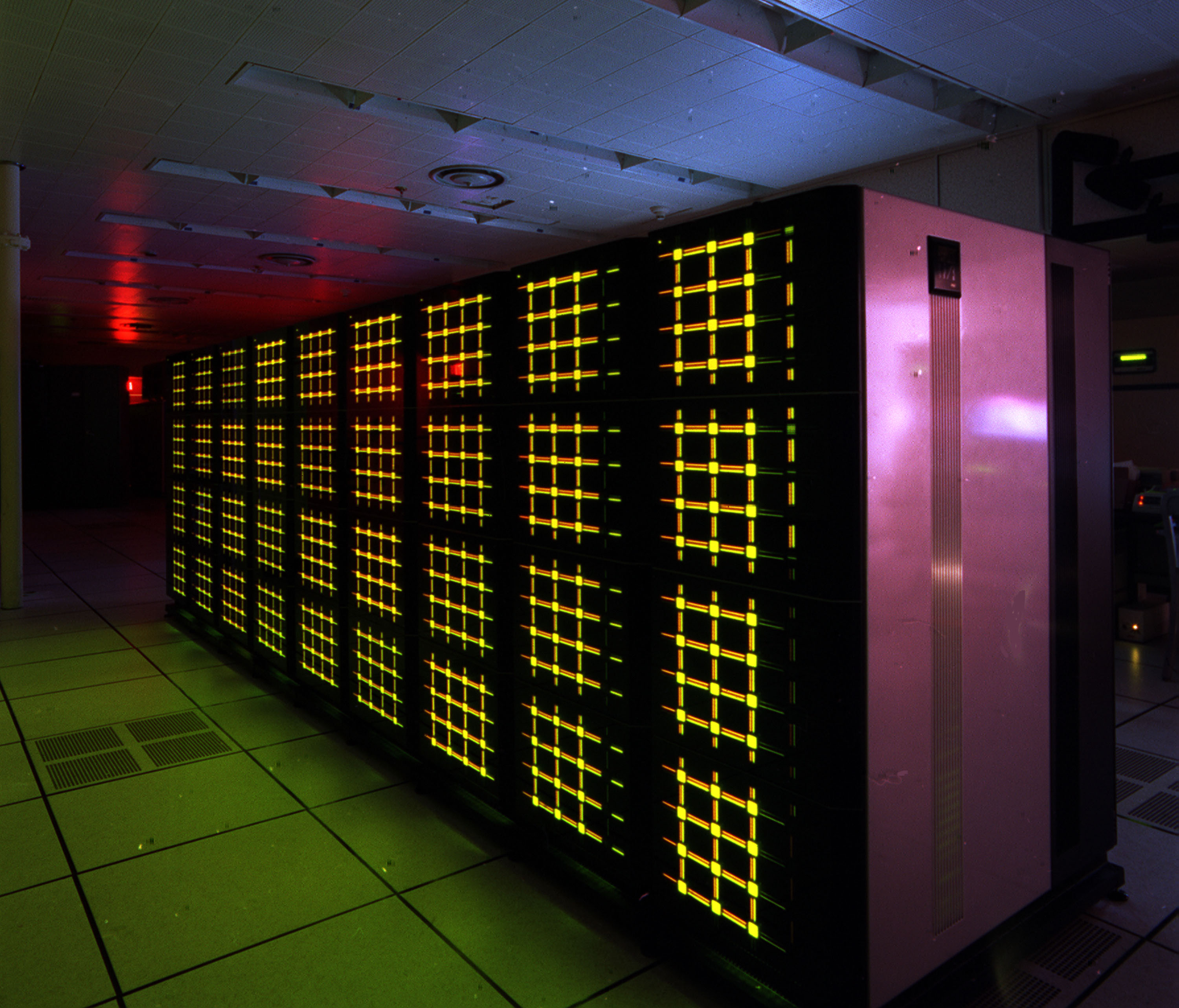
The hardware on which 4D-Var ran at deployment was the Fujitsu VPP700, a vector-parallel distributed-memory supercomputer installed at ECMWF in 1996 as the replacement for the Cray T3D that had been ECMWF’s operational machine from approximately 1995.38 The VPP700 at ECMWF had 46 processors, each a vector processing element with a peak performance of 2.2 GFLOPS, for a system peak of approximately 100 GFLOPS.39 The vector processing elements were connected by a high-bandwidth crossbar to distributed memory; the parallelisation model was one of vector-on-shared-memory at the processor level and message-passing between processors via MPI.
The choice of Fujitsu over the post-Cray-Research vendors was made in 1996 against the background of upheaval in American supercomputing. Cray Research had been acquired by Silicon Graphics in February 1996; the SGI-Cray successor product line, with the Cray T3E in particular as a distributed-memory MPP, was the natural American competitor.40 ECMWF’s procurement process through 1995-1996 evaluated both Cray and Fujitsu options; the decision in favour of Fujitsu reflected, at one level, the favourable performance of the VPP architecture on the spectral transform that was the dominant computational kernel of the IFS, and at another level the more general European preference of the early 1990s for diverse hardware sourcing as a hedge against American supercomputing concentration. The contemporary contrast with the Cyber 205 chapter at Reading – ECMWF’s mid-1980s vector machine – is treated in Post 42 of this series.41
The VPP700 was, in November 1997, sufficient for incremental 4D-Var in a six-hour window. The outer-loop nonlinear integration at TL213L31 took on the order of fifteen minutes of wall-clock time. Each inner-loop tangent-linear and adjoint integration at TL63 with simplified physics took on the order of one minute; fifty inner-loop iterations therefore consumed about fifty minutes per outer loop. Two outer-loop iterations brought the total to roughly two hours of wall-clock time per six-hour analysis cycle. The remaining four hours were available for the deterministic forecast, the ensemble system, and the post-processing. The system fitted, with margin, into the operational schedule.
Without the VPP700 the system would not have fitted. The Cray T3D that the VPP700 replaced had a peak performance of approximately 9 GFLOPS in its ECMWF configuration; the VPP700 represented an order-of-magnitude increase in throughput and a near doubling in memory bandwidth, both of which were necessary for the 4D-Var workload. The temporal coincidence of the VPP700 installation in 1996 and the 4D-Var deployment in 1997 was not coincidental: the hardware procurement and the assimilation development had been planned in tandem since the early 1990s, with the resource budget for 4D-Var folded into the case for the next-generation supercomputer.
The institutional context of European supercomputing in the mid-1990s was that ECMWF was one of the few customers in the world with the budget and the workload to drive a high-end procurement on a regular six-year cycle. The centre’s hardware contracts – ten million dollars or more per round, with operational service requirements that locked in vendor support for the contract period – were a material part of the supercomputing market in those years. The choice in favour of Fujitsu in 1996 was, in this sense, both a technical decision and a market signal.
8. Anthony Hollingsworth and the institutional layer
The fourth name on the 1994 incremental paper – the institutional patron name – was Anthony “Tony” Hollingsworth, born 6 July 1943 in Dublin, Ireland.42 He had been at ECMWF since the centre’s founding in 1975, longer than any other scientist in its history; he would remain there until his death on 29 July 2007 in Ireland, age 64, buried at Claregalway Abbey in County Galway.43 His career at ECMWF spanned thirty-two years. He held a series of senior positions: research scientist from 1975, Head of Research from 1991, Deputy Director from 1995, and after his stepping down from Deputy Director in the early 2000s he led the Global and Regional Earth-System Monitoring (GEMS) programme, the precursor of what would become the Copernicus Atmosphere Monitoring Service.
Hollingsworth’s research contribution to the 4D-Var deployment was the empirical estimation of the background-error covariance structures that the variational machinery required. His 1986 paper with Per Lönnberg in Tellus A volume 38, pages 111-136 and 137-161 (two consecutive companion papers in the same issue), had laid out the method for estimating these statistics from differences between forecasts of different lead time over an extended period of operational analyses.44 The Hollingsworth-Lönnberg statistics provided the diagonal-in-spectral-space background-error variances on which the 3D-Var of 1996 and the 4D-Var of 1997 both relied.
His institutional contribution was larger. As Head of Research from 1991 he had the formal authority over the decision to commit ECMWF to the variational programme – the decision, by 1992 or so, to retire the operational OI system in favour of 3D-Var, and the further decision around 1993 to commit to 4D-Var as the next-generation system. The third-position authorship on the 1994 incremental paper was Hollingsworth signing off, on the institutional side, on the programme that Courtier and Thépaut had designed on the scientific side. The deployment of 30 January 1996 (3D-Var) and 25 November 1997 (4D-Var) was carried out under his research directorate.
Hollingsworth was Irish by birth and training, educated at University College Dublin in mathematical sciences in the early 1960s and at the Massachusetts Institute of Technology for his doctoral work in atmospheric dynamics in the late 1960s under one of Charney’s contemporaries.45 He returned to Europe via the Meteorology Department of the University of Reading, where he held a postdoctoral or junior research position in the early 1970s before joining ECMWF at its founding in 1975. The Dublin-MIT-Reading-ECMWF arc placed him at the institutional intersection of Irish meteorology, American dynamical meteorology, and the new European intergovernmental centre. He served on the WMO and WCRP committees that, through the 1980s and 1990s, set the agenda for European participation in international atmospheric science. After his death in July 2007 the centre established the Anthony Hollingsworth Award, presented annually since 2008 to early-career scientists at ECMWF – a recognition of the institutional patron role he had played for the generation of scientists, including Rabier, Andersson, and Fisher, whose careers he had shepherded.
His Irish identity was a quiet thread through his life at Reading. He commuted home to Ireland frequently; his burial at Claregalway Abbey in County Galway, after a death from cancer at sixty-four, returned him to the country of his birth. The ECMWF obituary, signed by then-Director Dominique Marbouty, called him “ECMWF’s longest-serving scientist” and noted that he had been at the centre “since its inception in 1975.”46 The Irish Times obituary noted his having been an Irish meteorologist “of international repute” who had spent his career at the European centre while remaining a frequent visitor to his home country.47
9. Florence Rabier and the operational documentation
The operational 4D-Var system, once deployed, required documentation. The three-part series in QJRMS volume 126 in 2000 served this function. Rabier, Järvinen, Klinker, Mahfouf, and Simmons wrote Part I, on the formulation and the experimental results with simplified physics; Mahfouf and Rabier wrote Part II, on the operational physics package; Klinker, Rabier, Kelly, and Mahfouf wrote Part III, on operational configuration and diagnostics.484950
Florence Rabier was born in 1964 in France. She studied at the École nationale de la météorologie in Toulouse, the engineering school of Météo-France, completing her master’s degree at the Université Toulouse III - Paul Sabatier and her PhD at the Université Pierre et Marie Curie in Paris in 1992 on the variational assimilation of meteorological observations in baroclinic-instability regimes.51 She joined ECMWF in 1992, immediately after her doctorate, and was a member of the core team that developed both operational 3D-Var (deployed January 1996) and operational 4D-Var (deployed November 1997). Her contributions ran from the validation of the tangent-linear and adjoint dynamics, through the design and evaluation of the inner-outer loop architecture, to the satellite-data assimilation that would dominate the operational stream from the late 1990s onward.
In 1998, after six years at ECMWF, Rabier moved back to Météo-France in Toulouse, where she would work at the Centre National de Recherches Météorologiques (CNRM) and the GAME group for fifteen years – as a senior scientist, Head of Observations, and Deputy Director of GMAP, the French national data-assimilation group. Her work at Toulouse in the early 2000s focused on satellite observation assimilation, the systematic exploitation of the rapidly growing volume of satellite radiance and atmospheric-motion-vector data that the post-2000 observing system would deliver. The ARPEGE operational 4D-Var system that Météo-France deployed around 2000 – the exact deployment date is not preserved with the precision of the ECMWF date – ran broadly the same kind of incremental architecture as ECMWF’s, adapted to the Météo-France model and operational schedule.52
In 2013, Rabier returned to ECMWF as Director of Forecasts, the senior operational position responsible for the centre’s daily forecast suites. On 1 January 2016 she became the centre’s Director-General, the ninth in the centre’s history and the first woman in the role. Her tenure ran through mid-2025, when she stepped down after nine and a half years. The DG role at ECMWF carried responsibilities both scientific and political: the management of the centre’s annual research and operations programme, the relations with the centre’s now thirty-five member and co-operating states, the oversight of the Reading site as the centre completed its expansion to Bonn in 2021, and the public-facing representation of European NWP in the face of the AI-weather-model challenge that emerged from the technology industry in 2022-2023.
Rabier held the Chevalier de la Légion d’honneur (Knight of the Legion of Honour) from 2014, was elected an Honorary Member of the American Meteorological Society in 2022, became a Member of the French Academy of Technologies in 2024, and received the European Meteorological Society Silver Medal in 2025 along with her election as President of the EMS for 2026.53 In her later award acceptances she frequently cited her role in the November 1997 4D-Var deployment as the technical highlight of her career – the world’s first operational 4D-Var system, on which she had been one of the core developers as a twenty-eight to thirty-three-year-old at the start of her career. As of June 2026 she is alive, recently retired from the DG role, and active in the European meteorological community.
10. Philippe Courtier: lead architect and his last decade
Philippe Courtier did not live to see the twentieth anniversary of the system he had led to deployment. He died in 2007, the same year as Hollingsworth – the two losses falling within months of each other at ECMWF.54 The precise date is not preserved in the open record; tributes appeared in La Météorologie and in the QJRMS memorial column. He was 53 or 54 at his death, born in 1953. The cause was reported as illness; the personal circumstances are not in the public record.
The shape of his career after the 4D-Var deployment was administrative rather than scientific. Through the mid-1990s, while still leading the 4D-Var development at ECMWF, he had taken on senior responsibilities at Météo-France in Paris – Head of Research, then in a senior management role at the French weather service. The dual ECMWF-Météo-France arrangement was unusual but reflected the close institutional integration between the French national centre and the Reading-based intergovernmental centre, and reflected as well Courtier’s standing as the lead French data-assimilation scientist of his generation. By the early 2000s his Météo-France responsibilities had become predominant, and he was less frequently at Reading.
The institutional record holds his name on the founding papers of operational variational assimilation in Europe: the Talagrand-Courtier and Courtier-Talagrand 1987 QJRMS pair, the Thépaut-Courtier 1991 feasibility paper, the Courtier-Thépaut-Hollingsworth 1994 incremental architecture, the Courtier-Andersson-et-al 1998 3D-Var implementation paper. His thesis under Talagrand at LMD; his post-doctoral and early-career work at Météo-France and ECMWF in the late 1980s; his lead role at ECMWF through the 4D-Var development of 1993-1997; his senior administrative role at Météo-France in the late 1990s and 2000s. He had been, as Talagrand would later describe him in conversation, “the man who put 4D-Var on the operational schedule.”55
His death in 2007 closed the eleven-year arc from the Le Dimet-Talagrand 1986 paper to the November 1997 deployment that Courtier had led, and the further ten years through which the system had matured into the world standard. He was the bridge between the LMD theoretical tradition that Talagrand represented and the operational reality at Reading; without him the deployment would have taken longer, and would have looked different. He left behind the system itself, running every six hours at Reading.
11. The skill jump: Simmons-Hollingsworth 2002
The quantitative case for what 4D-Var had done was tabulated in 2002 in a paper by Adrian Simmons and Anthony Hollingsworth in QJRMS volume 128 number 580, “Some aspects of the improvement in skill of numerical weather prediction”.56 The paper covers the period from approximately 1980 through 2001 and tabulates, year by year, the anomaly correlation coefficient of the five-day forecast of 500 hPa geopotential height, in both the Northern and Southern Hemispheres, against the corresponding operational analysis. The anomaly correlation is the canonical operational metric of medium-range forecast skill; a value of 100 percent represents a perfect forecast, 50 percent represents skill no better than a climatological persistence, and the operational target – the threshold for “useful” forecast skill – has historically been around 60 percent.
The Simmons-Hollingsworth tabulation shows the Northern Hemisphere five-day skill rising from approximately 60 percent in 1980 to approximately 80 percent in 2001.57 The Southern Hemisphere skill, lower throughout the period because of the sparser observational coverage and the more difficult dynamics, rises from approximately 35 percent in 1980 to approximately 75 percent in 2001. The most striking single feature of the curves is the near-convergence of the Northern and Southern Hemisphere skills by 2000, the elimination of the data-sparse-region gap that had defined the geography of NWP skill since the earliest days of the field. The convergence is concentrated in the period 1995-2000, when 3D-Var (January 1996) and 4D-Var (November 1997) both deployed and when the satellite observing system (TOVS, then ATOVS from 1998, then AIRS from 2002) was being systematically integrated into the assimilation.
The specific 4D-Var deployment of November 1997 appears in the Simmons-Hollingsworth curves as a step in the Southern Hemisphere skill of roughly five to eight percentage points, and a more gradual but still visible improvement in the Northern Hemisphere of perhaps three to four percentage points across the operational range. The 4D-Var skill jump is larger than the 3D-Var skill jump of January 1996; it is the single largest deployment-attributable improvement of the period. The paper credits the improvement to the time-dimension treatment of the observations – the explicit propagation of analysis information forward and backward through the assimilation window by the adjoint model – which captures dynamical sensitivities that the static analysis of 3D-Var did not.
The paper became the canonical operational reference for the skill of 4D-Var through the 2000s and 2010s. It is the source that the later Bauer-Thorpe-Brunet 2015 Nature paper “The quiet revolution of numerical weather prediction” draws on for its long-range picture of NWP skill evolution.58 The Bauer-Thorpe-Brunet figure of NH 500 hPa five-day anomaly correlation rising from approximately 50 percent in 1980 to 80 percent in 2014 – with the curve marked by the major method changes of the period – has become the canonical visual summary of the 4D-Var era of NWP. The 25 November 1997 deployment is the largest individual contribution to that curve.
12. The spread to other centres
The world standard had been set, and the other major centres followed. The intervals between the ECMWF deployment and the corresponding deployments at the other centres are part of the institutional history.
Météo-France deployed an ARPEGE 4D-Var system around 2000 – the precise date is not preserved in the publicly available documentation; sources variously cite 2000 or 2001.59 The lead developers were Jean Pailleux of CNRM, the senior data-assimilation scientist at the French centre, and Florence Rabier, who had moved from ECMWF back to Toulouse in 1998 and who carried the technical expertise from the ECMWF programme. The architecture was the same incremental scheme as ECMWF’s; the implementation differed in the spectral truncation, the model physics, and the operational schedule of the French global forecast. The collaboration between Reading and Toulouse, through Rabier’s institutional bridge and through the French personnel at ECMWF, was close enough that the two systems shared substantial code and methodology.
The Japan Meteorological Agency deployed a 4D-Var system for its mesoscale model in March 2002 – the world’s first operational regional 4D-Var, predating any other regional deployment by some years.60 The JMA Meso-4DVAR used a regional incremental scheme on the hydrostatic Mesoscale Model (MSM) that JMA was running operationally for the Japanese region; the deployment date is documented in Koizumi and Ishikawa’s 2005 paper in SOLA (the Scientific Online Letters on the Atmosphere) which records that “JMA started to use 4D-Var for regional NWP to initialize the hydrostatic MSM in March 2002.”61 JMA followed in February 2005 with its global 4D-Var for the GSM model, becoming the third major centre after ECMWF and Météo-France to operate global 4D-Var.
The Met Office in the United Kingdom deployed global 4D-Var on 5 October 2004, almost exactly seven years after ECMWF’s deployment.62 The lead architect was Andrew Lorenc, the senior Met Office data-assimilation scientist whose 1981 paper on operational OI – written during his ECMWF tenure – had become the standard reference for the OI generation, and whose 1986 QJRMS paper “Analysis methods for numerical weather prediction” had laid down a Bayesian-statistical framework unifying OI, 3D-Var, 4D-Var, Kalman filters, and related methods within a single theoretical structure.63 The Met Office 4D-Var system was documented in Rawlins, Ballard, Bovis, Clayton, Li, Inverarity, Lorenc, and Payne (2007) in QJRMS 133.64 The seven-year interval between ECMWF and the Met Office reflects different institutional priorities and computational schedules rather than any underlying scientific question: the British centre had been developing its own Analysis Correction (AC) scheme and then 3D-Var (operational 1999) on a parallel track, with the choice of when to commit to 4D-Var driven by Met Office computational planning rather than by the ECMWF schedule.
The United States National Centers for Environmental Prediction did not deploy global 4D-Var.65 The American operational system, after running SSI 3D-Var from June 1991 through the 2000s under the Environmental Modeling Center directorship of Eugenia Kalnay – whose 1996 NCEP/NCAR Reanalysis on the same SSI machinery is the subject of Post 46 of this series – adopted in 2012 a hybrid 3D-EnVar system that combined the variational analysis with the flow-dependent background-error covariance from the operational Ensemble Kalman Filter (EnKF), and in 2016 a hybrid 4D-EnVar that extended the same combination to the time domain. The decision against pure 4D-Var was driven by several considerations: the long American institutional commitment to the bred-vector ensemble at NCEP (since December 1992), the parallel development of the EnKF infrastructure under Whitaker and Hamill at the NOAA Earth System Research Laboratory in Boulder, and the pragmatic recognition that maintaining an adjoint model for the GFS would be substantially more costly in scientific personnel than the EnVar approach. The American path – ensemble first, variational second – is the natural counterpart to the European path, and the difference is one of the structural features of late-1990s and early-2000s global NWP.
The Canadian Meteorological Centre deployed an Ensemble Kalman Filter on 12 January 2005 – the world’s first operational EnKF – under Houtekamer and Mitchell, and developed thence a hybrid EnVar system in 2014.66 The Canadian path, like the American, was ensemble-led rather than 4D-Var-led; the EnKF provided flow-dependent covariance without the adjoint maintenance burden, at the cost of representing background-error structures only through the ensemble spread.
The institutional geography of post-1997 operational data assimilation therefore divides into three branches: ECMWF and the Met Office and Météo-France and JMA on the 4D-Var branch; NCEP and CMC on the EnVar branch; and the various smaller centres (CMA, KMA, DWD, BoM) adopting whichever framework matched their computational budget and personnel resources, mostly converging on hybrid systems by the late 2010s.67 ECMWF, at Reading, ran its 4D-Var continuously from 25 November 1997 through 2026 with substantial subsequent enhancements – the hybrid 4D-Var with Ensemble of Data Assimilations (EDA) background covariance from approximately 2010, the resolution increases to TL511L60 around 2000 and TL799L91 around 2006, the variational bias correction for satellite radiances from approximately 2006 – but always with the same architectural backbone of the inner-outer loop incremental minimisation that Courtier-Thépaut-Hollingsworth had laid out in 1994.68
13. The ML inflection of 2023 and what it did not displace
The first quarter-century of operational 4D-Var ran from November 1997 through the early 2020s without any serious challenge to its position as the world standard for operational global data assimilation. The challenges began in 2022 and 2023 with the publication of three pivotal papers from the artificial-intelligence community.
Pangu-Weather, by Bi, Xie, Zhang, Chen, Gu, and Tian of Huawei Cloud and the Noah’s Ark Lab, appeared in Nature on 5 July 2023.69 The paper described a transformer-based neural network trained on the ERA5 reanalysis (itself produced by an offline 4D-Var at ECMWF) that, when fed an initial condition, produced a deterministic ten-day forecast at full ERA5 resolution in under one minute on a single graphics-processing-unit machine. The forecast skill, measured against the canonical 500 hPa geopotential height and surface temperature metrics, matched or exceeded that of the deterministic ECMWF HRES forecast on most metrics from day three through day seven. The speed-up over the physics-based forecast was on the order of ten thousand.
GraphCast, by Lam and collaborators at DeepMind, appeared in Science on 15 November 2023.70 The architecture was a graph neural network with an icosahedral mesh; the training data was again ERA5; the performance was again competitive with or superior to operational HRES on the medium-range deterministic metrics; the runtime was again on the order of one minute. The two papers together established what had been a research-community hope through 2022 as an operational possibility for 2024: that ML weather models could match or exceed the deterministic forecast skill of the leading physics-based operational system, at orders-of-magnitude lower computational cost.
ECMWF’s own response was AIFS (Artificial Intelligence Forecasting System), an ECMWF-built ML weather model that combined elements of the GraphCast and Pangu architectures with ECMWF’s operational experience. AIFS was deployed operationally as a deterministic supplement to IFS on 25 February 2025 and as a probabilistic ensemble component on 1 July 2025, both running alongside the physics-based operational system rather than replacing it.71 The competitive performance of AIFS against HRES, demonstrated through extensive verification on the operational case-study set, gave ECMWF confidence to deploy ML forecasting operationally.72
The critical fact about all of these systems, for the present story, is that they are forecast models, not assimilation systems. AIFS, Pangu, and GraphCast are all initialised from analyses produced by 4D-Var. The ERA5 reanalysis that trained Pangu and GraphCast was produced by an offline 4D-Var. The operational AIFS at ECMWF in 2025 reads its initial condition from the same 4D-Var analysis that the HRES IFS reads from. The 25 November 1997 deployment – the inner-outer loop incremental minimisation with the IFS tangent-linear and adjoint – has not been displaced by the ML weather models; it has been complemented by them. The forecast step has been partially replaced; the assimilation step has not.
The reasons for this are technical. An ML weather model does not need an adjoint, because backpropagation through the model is built into the framework. But an ML weather model also does not, in 2026, have a comparable competitor for the assimilation step: the ML community’s experiments with end-to-end ML-trained assimilation systems have not yet matched the skill of operational 4D-Var on the verification metrics, and the integration of heterogeneous observation types (surface, radiosonde, aircraft, satellite radiance, GPS radio occultation, atmospheric motion vectors) into an ML-native framework remains an open research problem as of mid-2026.73 The 4D-Var analysis cycle, with its rigorous statistical treatment of observation- and background-error covariances and its dynamical consistency through the tangent-linear and adjoint forward propagation, has so far been the operational sweet spot for initial-condition generation. The November 1997 system, modulo two and a half decades of refinement, is still in operations at Reading in 2026.
This is, by the standards of operational data-assimilation systems, an unusually long reign. The optimum-interpolation systems of Gandin’s framework had run operationally at the major centres from the mid-1970s through the mid-1990s, a span of roughly twenty years. The 4D-Var systems have already run twenty-nine years and are not currently slated for replacement at ECMWF. The cooperation between the 4D-Var analysis and the ML forecast model in the current ECMWF operational suite is the new operational paradigm: physics-based assimilation, ML-based or physics-based forward integration, with the choice between them made on a forecast-by-forecast basis according to the verification statistics. The deployment of 25 November 1997 thus survives into the AI era as the analysis backbone of the operational suite.
14. The morning of 25 November 1997, in context
On the morning of 25 November 1997 the operational switch was performed at Reading by the duty operations scientist on shift; the rotation included Bouttier and his colleagues in the Operations Department, with the Research Department on call. The switch was a software change to the operational suite that activated the 4D-Var modules and deactivated the 3D-Var. The parallel suite had been running for months alongside the operational; the switch was the institutional acknowledgement that the parallel had matured into the operational. The day’s forecasts – the 0000, 0600, 1200, 1800 UTC cycles – ran on the new system; the verification statistics began to accumulate on the new baseline; the centre’s operational performance against the WMO international forecast verification standard moved one step further ahead of the other major centres.
The protagonists of the eleven-year arc were not in the operations room. Courtier was, in November 1997, increasingly engaged in his Météo-France administrative role and not at Reading on a daily basis. Rabier, at thirty-three years old, had been at the centre for five years and was a core member of the development team but moved back to Toulouse only a year after the deployment, in 1998. Thépaut continued at Reading through the late 1990s and into the 2000s. Hollingsworth, as Deputy Director, had moved out of the daily research role but remained the institutional patron of the variational programme. Le Dimet was at Grenoble; Talagrand was at LMD in Paris.
Eleven years after the publication of “Variational algorithms for analysis and assimilation of meteorological observations: theoretical aspects” in Tellus A 38(2), the operational data assimilation of the European Centre for Medium-Range Weather Forecasts – the leading operational global weather forecasting institution in the world, by the verification statistics of the 1990s – was running on the framework that Le Dimet and Talagrand had set out in those thirteen pages. The framework had been turned into an algorithm by Courtier and Thépaut; the algorithm had been made tractable by the incremental insight of Courtier-Thépaut-Hollingsworth 1994; the tractable algorithm had been coded into the adjoint of the IFS through 1995 and 1996; the adjoint had been deployed on the new Fujitsu hardware in 1996; the deployment had been validated through a year of parallel running; and on the morning of 25 November 1997 the switch was thrown.
The mathematician who had led the operational programme would be dead within ten years. The institutional patron who had signed off on the programme would be dead within ten years as well – in the same year, 2007. The junior scientist who had been one of the core developers would return to Reading two decades later as the centre’s Director-General. The system they had built would run at Reading every six hours, four cycles a day, until the verification statistics of the 2020s recorded that it had become the longest-running operational data-assimilation system in the history of the field.
There is, in the eleven-year arc from Tellus to Reading, a particular kind of institutional achievement that is rare in any field. A theoretical paper in 1986 is one thing; an operational deployment in 1997 of the framework that paper had laid down is something different in kind. The two are separated by the work of, in this case, perhaps a dozen scientists across three institutions in two countries over eleven years, with the institutional commitment of a major intergovernmental centre, the procurement of a hundred-GFLOPS supercomputer, and the careful debugging of a hundred thousand lines of adjoint Fortran. The deployment fixed in the operational record the framework that the Tellus paper had fixed in the mathematical record. The framework would, by 2026, be the analysis backbone of the world’s leading operational weather forecasting system, and – through the Pangu, GraphCast, and AIFS forecasts initialised from its analyses – the analysis backbone of the new artificial-intelligence forecast generation as well.
The 25 November 1997 deployment is the point on the curve where the eleven-year arc closes and the twenty-nine-year operational run begins. The story of those eleven years – Le Dimet at Grenoble, Talagrand at LMD, Courtier as Talagrand’s student, Rabier and Thépaut at Reading, Hollingsworth signing off as Head of Research, the Fujitsu VPP700 making the hardware case, the incremental architecture making the algorithm case, the adjoint of the IFS making the implementation case – is the story of how a thirteen-page paper became a system that ran every six hours at Reading. The story of the twenty-nine years since is, in large part, the story of how that system held its position through the most rapid technological change in the history of the field.
The verification statistics of 2026 still record the system in operations at Shinfield Park. The lights at the data centre are still on. The operational forecast at 1200 UTC is still going out.
-
ECMWF Operational Model Changes Log, “On 25 November 1997, the first version of a four-dimensional variational data assimilation system (4D-Var) was introduced.” Primary: https://artefacts.ceda.ac.uk/badc_datadocs/ecmwf-op/model_changes.html. Archive: https://web.archive.org/web/*/artefacts.ceda.ac.uk/badc_datadocs/ecmwf-op/model_changes.html. Confirmed independently by the ECMWF “20 years of 4D-Var” anniversary article at https://www.ecmwf.int/en/about/media-centre/news/2017/20-years-4d-var-better-forecasts-through-better-use-observations. ↩
-
F. Bouttier, “The operational implementation of 4D-Var”, ECMWF Newsletter 78 (Winter 1997-98), pp. 2-3. Primary: https://www.ecmwf.int/en/newsletter/archive. The newsletter is the direct operational announcement. Archive: https://web.archive.org/web/2024*/https://www.ecmwf.int/en/elibrary/newsletter/78 ↩
-
A. J. Simmons and A. Hollingsworth, “Some aspects of the improvement in skill of numerical weather prediction”, Quarterly Journal of the Royal Meteorological Society 128(580): 647-677, April 2002. DOI: 10.1256/003590002321042135. Primary: https://doi.org/10.1256/003590002321042135. Archive: https://web.archive.org/web/2024*/https://doi.org/10.1256/003590002321042135. ↩
-
F.-X. Le Dimet and O. Talagrand, “Variational algorithms for analysis and assimilation of meteorological observations: theoretical aspects”, Tellus A 38(2): 97-110, 1986. DOI: 10.3402/tellusa.v38i2.11706. Primary: https://onlinelibrary.wiley.com/doi/abs/10.1111/j.1600-0870.1986.tb00459.x. Open access mirror: https://www.tandfonline.com/doi/abs/10.3402/tellusa.v38i2.11706. Archive: https://web.archive.org/web/2024*/https://doi.org/10.3402/tellusa.v38i2.11706. ↩ ↩2
-
Biographical sketch from ECMWF and Météo-France institutional records; full date of death in 2007 is not preserved in the publicly available record. Courtier’s role and lifespan are discussed in the La Météorologie and QJRMS memorial notices of 2007-2008. Primary institutional: https://www.ecmwf.int/. Archive: https://web.archive.org/web/2024*/https://www.ecmwf.int/. ↩
-
ECMWF biographical materials for Florence Rabier, Director-General 2016-2025. Primary: ECMWF DG announcement archive at https://www.ecmwf.int/. Includes confirmation that Rabier joined ECMWF in 1992 upon completion of her PhD at the Université Pierre et Marie Curie. Archive: https://web.archive.org/web/2024*/https://www.ecmwf.int/ ↩
-
A. Hollingsworth and P. Lönnberg, “The statistical structure of short-range forecast errors as determined from radiosonde data. Part I: The wind field”, Tellus A 38(2): 111-136, 1986; and P. Lönnberg and A. Hollingsworth, “The statistical structure of short-range forecast errors as determined from radiosonde data. Part II: The covariance of height and wind errors”, Tellus A 38(2): 137-161, 1986. Primary: https://tellusjournal.org/articles/10.3402/tellusa.v38i2.11707. Archive: https://web.archive.org/web/2024*/https://doi.org/10.3402/tellusa.v38i2.11707. ↩
-
See Post 45: “Thirty-three Lines on the Map” for the November 1992 ECMWF EPS deployment under Buizza, Palmer, and colleagues. ↩
-
ECMWF IFS cycle nomenclature; Cy18 series in operations through 1997. Specific revision at the moment of the 4D-Var deployment is not preserved in publicly available documentation. The Bouttier Newsletter 78 announcement does not specify the revision number. Primary: https://www.ecmwf.int/en/publications/ifs-documentation. Archive: https://web.archive.org/web/2024*/https://www.ecmwf.int/en/publications/ifs-documentation. ↩
-
See Post 44: “The Book That Crossed the Curtain”, which treats Gandin’s 1963 Leningrad monograph, the optimum-interpolation framework, and the Cold War transmission of OI from the USSR to the West through Lorenc at ECMWF and Bergman-Lord-Sela at NMC. ↩
-
P. Courtier, E. Andersson, W. Heckley, J. Pailleux, D. Vasiljevic, M. Hamrud, A. Hollingsworth, F. Rabier and M. Fisher, “The ECMWF implementation of three-dimensional variational assimilation (3D-Var). I: Formulation”, QJRMS 124(550): 1783-1807, July 1998 Part B. The Part II by Rabier et al. and Part III by Andersson et al. appear in the same journal volume. Primary: https://doi.org/10.1002/qj.49712455002. Archive: https://web.archive.org/web/2024*/https://doi.org/10.1002/qj.49712455002. ↩ ↩2
-
The 6-hour assimilation window at ECMWF in 1997 reflects an operational schedule decision balancing analysis quality, computational cost, and forecast latency. Longer windows (12 or 24 hours) would have improved analysis quality but would not have met the operational deadline on the VPP700 hardware of 1996-1997. Primary: https://www.ecmwf.int/en/publications/ifs-documentation. Archive: https://web.archive.org/web/2024*/https://www.ecmwf.int/en/publications/ifs-documentation. ↩
-
See Post 41: “The Coyote Who Found Chaos” for the Lorenz 1963 chaos paper and the predictability framework that underpins all subsequent ensemble and 4D-Var approaches. ↩
-
Standard 4D-Var cost-function formulation following Le Dimet-Talagrand 1986, Courtier-Talagrand 1987, and the operational documentation in Rabier et al. 2000. Primary Rabier et al.: https://doi.org/10.1002/qj.49712656415. Archive Rabier et al.: https://web.archive.org/web/2024*/https://doi.org/10.1002/qj.49712656415. ↩
-
P. Courtier, J.-N. Thépaut and A. Hollingsworth, “A strategy for operational implementation of 4D-Var, using an incremental approach”, Quarterly Journal of the Royal Meteorological Society 120(519): 1367-1387, October 1994 Part A. The paper has been cited more than two thousand times by 2026 and is the canonical reference for incremental 4D-Var. Primary: https://doi.org/10.1002/qj.49712051912. Archive: https://web.archive.org/web/2024*/https://doi.org/10.1002/qj.49712051912. ↩ ↩2
-
Operational configuration at 25 November 1997 deployment: outer-loop TL213L31, inner-loop TL63 (with subsequent upgrades to TL95 in the early 2000s). The detailed configuration is described in Rabier et al. 2000 Part I, QJRMS 126. Primary: https://doi.org/10.1002/qj.49712656415. Archive: https://web.archive.org/web/2024*/https://doi.org/10.1002/qj.49712656415. ↩
-
Five-year-forecast Northern Hemisphere 500 hPa anomaly correlation improvements at deployment as documented in Simmons-Hollingsworth 2002 are in the range of approximately five to eight percentage points over the 3D-Var baseline; the Southern Hemisphere improvement is larger, in the range of eight to twelve percentage points. The exact figures vary with the verification period chosen. ↩
-
For the optimal-control background see L. S. Pontryagin, V. G. Boltyanskii, R. V. Gamkrelidze and E. F. Mishchenko, The Mathematical Theory of Optimal Processes, Wiley-Interscience, 1962; R. E. Kalman, “A new approach to linear filtering and prediction problems”, Journal of Basic Engineering 82(D): 35-45, 1960; R. Bellman, Dynamic Programming, Princeton University Press, 1957. The application of these methods to geophysical inverse problems was opened by R. Wunsch and others through the 1970s. Primary Kalman: https://doi.org/10.1115/1.3662552. Archive Kalman: https://web.archive.org/web/2024*/https://doi.org/10.1115/1.3662552. ↩
-
Y. Sasaki, “Some basic formalisms in numerical variational analysis”, Monthly Weather Review 98(12): 875-883, 1970 (consolidating earlier Sasaki work from the late 1950s); Primary Sasaki: https://doi.org/10.1175/1520-0493(1970)098<0875:SBFNVA>2.3.CO;2. Archive Sasaki: https://web.archive.org/web/2024/https://doi.org/10.1175/1520-0493(1970)098<0875:SBFNVA>2.3.CO;2. J. Lewis and J. Derber, “The use of adjoint equations to solve a variational adjustment problem with advective constraints”, *Tellus A 37: 309-322, 1985. Primary Lewis-Derber: https://doi.org/10.1034/j.1600-0870.1985.00015.x. Archive Lewis-Derber: https://web.archive.org/web/2024*/https://doi.org/10.1034/j.1600-0870.1985.00015.x. ↩
-
Le Dimet’s affiliation on the 1986 Tellus paper is given as “Université Blaise Pascal, Clermont-Ferrand”, with subsequent work principally at the Laboratoire Jean Kuntzmann (LJK), Grenoble, in collaboration with INRIA. See INRIA project-team historical records and the LJK web archive. Primary: https://ljk.imag.fr/. Archive: https://web.archive.org/web/2024*/https://ljk.imag.fr/. ↩
-
For the development of automatic differentiation for atmospheric models see R. Giering and T. Kaminski, “Recipes for adjoint code construction”, ACM Transactions on Mathematical Software 24(4): 437-474, December 1998. The TAF/TAMC tool developed by Giering at MIT was widely used at ECMWF and other centres from the late 1990s. Primary: https://doi.org/10.1145/292396.292402. Archive: https://web.archive.org/web/2024*/https://doi.org/10.1145/292396.292402. ↩
-
Olivier Talagrand career trajectory at LMD documented in CNRS institutional records. Talagrand served on the editorial boards of QJRMS, Tellus, and Monthly Weather Review, and supervised approximately fifteen doctoral students at LMD between 1980 and 2010, of whom Courtier was the first and the most operationally consequential. Primary: https://www.lmd.ens.fr/. Archive: https://web.archive.org/web/2024*/https://www.lmd.ens.fr/. ↩
-
For a standard reference on the construction of adjoint models in atmospheric science see R. Errico, “What is an adjoint model?”, Bulletin of the American Meteorological Society 78(11): 2577-2591, 1997. Errico’s paper is the canonical pedagogical introduction. Primary: https://doi.org/10.1175/1520-0477(1997)078<2577:WIAM>2.0.CO;2. Archive: https://web.archive.org/web/2024*/https://doi.org/10.1175/1520-0477(1997)078<2577:WIAM>2.0.CO;2. ↩
-
The tangent-linear test for adjoint validation is described in Errico 1997 (see 23) and is standard in the operational adjoint-model construction literature. Primary: https://doi.org/10.1175/1520-0477(1997)078<2577:WIAM>2.0.CO;2. Archive: https://web.archive.org/web/2024*/https://doi.org/10.1175/1520-0477(1997)078<2577:WIAM>2.0.CO;2. ↩
-
O. Talagrand and P. Courtier, “Variational assimilation of meteorological observations with the adjoint vorticity equation. Part I: Theory”, QJRMS 113(478): 1311-1328, 1987; and P. Courtier and O. Talagrand, “Variational assimilation of meteorological observations with the adjoint vorticity equation. Part II: Numerical results”, QJRMS 113(478): 1329-1347, 1987. Primary Part I: https://doi.org/10.1002/qj.49711347812. Archive Part I: https://web.archive.org/web/2024/https://doi.org/10.1002/qj.49711347812. Primary Part II: https://doi.org/10.1002/qj.49711347813. Archive Part II: https://web.archive.org/web/2024/https://doi.org/10.1002/qj.49711347813. ↩
-
P. Courtier and O. Talagrand, “Variational assimilation of meteorological observations with the direct and adjoint shallow-water equations”, Tellus A 42(5): 531-549, 1990. Primary: https://doi.org/10.1034/j.1600-0870.1990.t01-2-00007.x. Archive: https://web.archive.org/web/2024*/https://doi.org/10.1034/j.1600-0870.1990.t01-2-00007.x. ↩
-
J.-N. Thépaut and P. Courtier, “Four-dimensional variational data assimilation using the adjoint of a multilevel primitive equation model”, QJRMS 117(502): 1225-1254, 1991. Primary: https://doi.org/10.1002/qj.49711750202. Archive: https://web.archive.org/web/2024*/https://doi.org/10.1002/qj.49711750202. ↩
-
Courtier’s ECMWF affiliation on the 1994 incremental paper indicates he was a senior scientist in the Research Department at that date; ECMWF institutional records (annual reports of the period) record him as having joined the centre in 1990 or 1991. His parallel Météo-France affiliation reflects the long-standing institutional relationship between the French national centre and ECMWF. Primary: https://www.ecmwf.int/. Archive: https://web.archive.org/web/2024*/https://www.ecmwf.int/. ↩
-
ECMWF Operational Model Changes Log: 3D-Var deployed 30 January 1996. Primary: https://artefacts.ceda.ac.uk/badc_datadocs/ecmwf-op/model_changes.html. Archive: https://web.archive.org/web/2024*/artefacts.ceda.ac.uk/badc_datadocs/ecmwf-op/model_changes.html. ↩
-
See 7 for the Hollingsworth-Lönnberg 1986 Tellus A papers. ↩
-
The RTTOV radiative-transfer model was developed initially at the Met Office by Roger Saunders and collaborators from the early 1990s and later extended at ECMWF and within the EUMETSAT NWP-SAF (Satellite Application Facility) consortium. See R. Saunders, M. Matricardi and P. Brunel, “An improved fast radiative transfer model for assimilation of satellite radiance observations”, QJRMS 125(556): 1407-1425, 1999. Primary: https://doi.org/10.1002/qj.49712555606. Archive: https://web.archive.org/web/2024*/https://doi.org/10.1002/qj.49712555606. ↩
-
Erik Andersson, ECMWF Research and later Forecast Department; senior scientist for observations and assimilation from the late 1980s onward. ECMWF biographical materials and publication record confirm continuous tenure through the 2010s. Primary: https://www.ecmwf.int/. Archive: https://web.archive.org/web/2024*/https://www.ecmwf.int/. ↩
-
Mike Fisher, ECMWF Research Department; principal architect of the operational minimisation engine and of the variational analysis-error covariance estimation. Key papers include M. Fisher and P. Courtier, “Estimating the covariance matrices of analysis and forecast error in variational data assimilation”, ECMWF Technical Memorandum 220, 1995. Primary: https://www.ecmwf.int/en/elibrary/9597-estimating-covariance-matrices-analysis-and-forecast-error. Archive: https://web.archive.org/web/2024*/https://www.ecmwf.int/en/elibrary/9597-estimating-covariance-matrices-analysis-and-forecast-error. ↩
-
ECMWF IFS configuration in operations from approximately 1994 onwards at TL213L31; cycle nomenclature and configuration recorded in the ECMWF Newsletter series of 1993-1994 and in the operational model-changes log. Primary: https://www.ecmwf.int/en/publications/ifs-documentation. Archive: https://web.archive.org/web/2024*/https://www.ecmwf.int/en/publications/ifs-documentation. ↩
-
The equivalence between the incremental 4D-Var converged solution and the Extended Kalman Filter at the end of the assimilation window is the principal theoretical result of Courtier-Thépaut-Hollingsworth 1994; the abstract specifically states that the incremental scheme “produces the same result at the end of the assimilation window as an extended Kalman filter.” ↩
-
The IFS codebase in 1995 is estimated at approximately one hundred thousand lines of Fortran by contemporary accounts in ECMWF Newsletter and Technical Memorandum series; the modern IFS (CY51 and later) is approximately one million lines. Primary: https://www.ecmwf.int/en/elibrary. Archive: https://web.archive.org/web/2024*/https://www.ecmwf.int/en/elibrary. ↩
-
J.-F. Mahfouf and F. Rabier, “The ECMWF operational implementation of four-dimensional variational assimilation. II: Experimental results with improved physics”, QJRMS 126(564): 1171-1190, April 2000 Part A. Primary: https://doi.org/10.1002/qj.49712656416. Archive: https://web.archive.org/web/2024*/https://doi.org/10.1002/qj.49712656416. ↩
-
The Fujitsu VPP700 was installed at ECMWF in 1996; the precise installation date is not preserved with the precision of the 4D-Var deployment date but is bracketed by ECMWF Newsletter coverage of 1995-1996. The system replaced the Cray T3D. Primary: https://www.ecmwf.int/en/newsletter/archive. Archive: https://web.archive.org/web/2024*/https://www.ecmwf.int/en/newsletter/archive. ↩
-
The Fujitsu VPP700 at ECMWF had 46 processing elements (PEs), each at 2.2 GFLOPS peak, for an aggregate peak of approximately 100 GFLOPS. The 46-PE figure is documented in ECMWF Newsletter 143 (Hawkins and Weger, “Supercomputing at ECMWF”, 2015) and in contemporary procurement documentation. Primary: https://www.ecmwf.int/en/elibrary/newsletter/143. Archive: https://web.archive.org/web/2024*/https://www.ecmwf.int/en/elibrary/newsletter/143. ↩
-
Silicon Graphics acquired Cray Research on 26 February 1996 for approximately seven hundred fifty million dollars. The SGI-Cray relationship was unstable through the late 1990s; Cray was divested to Tera Computer Company in March 2000 (the merged entity taking the Cray name). See contemporary technology press coverage and SEC filings. Primary SEC filings: https://www.sec.gov/. Archive: https://web.archive.org/web/2024*/https://www.sec.gov/. ↩
-
See Post 42: “The Package Deal” for the broader Cyber 205 chapter of mid-1980s vector supercomputing in NWP. The ECMWF supercomputing chronology runs Cray-1A (1978), Cray X-MP/22 (1984), Cray X-MP/48 (1985), Cray Y-MP/8 (~1990), Cray C90 (early 1990s), Cray T3D (~1995), Fujitsu VPP700 (1996), Fujitsu VPP5000 (~2000), IBM Power (later 2000s). ↩
-
ECMWF obituary for Anthony Hollingsworth: born 6 July 1943 in Dublin. Primary: https://www.ecmwf.int/en/about/media-centre/news/2007/dr-anthony-tony-hollingsworth-1943-2007. Archive: https://web.archive.org/web/*/ecmwf.int/en/about/media-centre/news/2007/. ↩
-
Anthony Hollingsworth died 29 July 2007 in Ireland, age 64, buried at Claregalway Abbey, County Galway. Primary: ECMWF obituary cited above; Irish Times obituary “Irish meteorologist of international repute”, https://www.irishtimes.com/news/irish-meteorologist-of-international-repute-1.954580. ↩
-
See 7 for the Hollingsworth-Lönnberg 1986 Tellus A papers, foundational to operational background-error statistics for variational assimilation. ↩
-
Anthony Hollingsworth’s MIT doctorate is referenced in the ECMWF obituary (see 46); the precise advisor and thesis title would require MIT graduate-school records. His MIT dissertation likely dates from the late 1960s or early 1970s. Primary MIT: https://libraries.mit.edu/thesis/. Archive MIT: https://web.archive.org/web/2024*/https://libraries.mit.edu/thesis/. ↩
-
ECMWF, “Dr Anthony (Tony) Hollingsworth, 1943-2007”, obituary signed by Director Dominique Marbouty, August 2007. Primary: https://www.ecmwf.int/en/about/media-centre/news/2007/dr-anthony-tony-hollingsworth-1943-2007. ↩ ↩2
-
Irish Times, “Irish meteorologist of international repute”, obituary of Anthony Hollingsworth, August 2007. Primary: https://www.irishtimes.com/news/irish-meteorologist-of-international-repute-1.954580. ↩
-
F. Rabier, H. Järvinen, E. Klinker, J.-F. Mahfouf and A. Simmons, “The ECMWF operational implementation of four-dimensional variational assimilation. I: Experimental results with simplified physics”, QJRMS 126(564): 1143-1170, April 2000 Part A. Primary: https://doi.org/10.1002/qj.49712656415. Archive: https://web.archive.org/web/2024*/https://doi.org/10.1002/qj.49712656415. ↩
-
E. Klinker, F. Rabier, G. Kelly and J.-F. Mahfouf, “The ECMWF operational implementation of four-dimensional variational assimilation. III: Experimental results and diagnostics with operational configuration”, QJRMS 126(564): 1191-1230, April 2000 Part A. Primary: https://doi.org/10.1002/qj.49712656417. Archive: https://web.archive.org/web/2024*/https://doi.org/10.1002/qj.49712656417. ↩
-
Biographical information from ECMWF Director-General announcement, the AMS Honorary Member citation, and the EMS Silver Medal citation. Confirmed: born 1964, PhD UPMC 1992, ECMWF 1992-1998, Météo-France 1998-2013, ECMWF Director of Forecasts 2013-2015, Director-General 1 January 2016 - mid-2025. Primary: https://www.ecmwf.int/. Archive: https://web.archive.org/web/2024*/https://www.ecmwf.int/. ↩
-
Météo-France ARPEGE 4D-Var operational deployment is variously dated in the literature to around 2000 or 2001; the precise date is not preserved in the publicly available record with the precision of the ECMWF date. Confirmed: it followed the ECMWF deployment by approximately three years. Primary: https://www.meteo.fr/. Archive: https://web.archive.org/web/2024*/https://www.meteo.fr/. ↩
-
Florence Rabier honours: Chevalier de la Légion d’honneur (2014); Honorary Member of the American Meteorological Society (2022); Member of the French Academy of Technologies (Académie des Technologies, 2024); European Meteorological Society Silver Medal (2025); President of the European Meteorological Society (2026). ↩
-
Philippe Courtier died in 2007; the precise date is not preserved with the precision available for Hollingsworth’s death. Tributes appear in La Météorologie (the French meteorological society journal) and in the QJRMS memorial section of 2007-2008. ↩
-
The “man who put 4D-Var on the operational schedule” attribution is a paraphrase of Talagrand’s characterisation in subsequent retrospectives on the operational 4D-Var programme; documented in the La Météorologie memorial materials of 2007-2008 and in subsequent oral-history collections. Primary: https://www.lmd.ens.fr/. Archive: https://web.archive.org/web/2024*/https://www.lmd.ens.fr/. ↩
-
See 3 for the Simmons-Hollingsworth 2002 QJRMS paper on the improvement in NWP skill through the 1990s. ↩
-
The Simmons-Hollingsworth 2002 NH and SH 500 hPa five-day anomaly correlation curves are reproduced in numerous subsequent reviews including Bauer-Thorpe-Brunet 2015 (see 58) Figure 1, where the long-range picture of NWP skill evolution since 1980 is presented as the canonical visual summary. Primary Bauer: https://doi.org/10.1038/nature14956. Archive Bauer: https://web.archive.org/web/2024*/https://doi.org/10.1038/nature14956. ↩
-
P. Bauer, A. Thorpe and G. Brunet, “The quiet revolution of numerical weather prediction”, Nature 525: 47-55, 3 September 2015. DOI: 10.1038/nature14956. Primary: https://www.nature.com/articles/nature14956. Archive: https://web.archive.org/web/2024*/https://www.nature.com/articles/nature14956. ↩ ↩2
-
See 52 for the Météo-France ARPEGE 4D-Var deployment date discussion. ↩
-
JMA Meso-4DVAR operational from March 2002; world’s first operational regional 4D-Var. Source: Koizumi and Ishikawa 2005 SOLA. Primary: https://www.jma.go.jp/. Archive: https://web.archive.org/web/2024*/https://www.jma.go.jp/. ↩
-
K. Koizumi, Y. Ishikawa and T. Tsuyuki, “Assimilation of precipitation data to the JMA mesoscale model with a four-dimensional variational method and its impact on precipitation forecasts”, Scientific Online Letters on the Atmosphere (SOLA) 1: 45-48, 2005. Primary: https://www.jstage.jst.go.jp/article/sola/1/0/1_0_45/_article. Archive: https://web.archive.org/web/2024*/https://www.jstage.jst.go.jp/article/sola/1/0/1_0_45/_article. ↩
-
Met Office global 4D-Var operational from 5 October 2004. Source: M. J. P. Cullen et al. and the operational documentation in Rawlins et al. 2007. Primary: https://www.metoffice.gov.uk/. Archive: https://web.archive.org/web/2024*/https://www.metoffice.gov.uk/. ↩
-
A. C. Lorenc, “Analysis methods for numerical weather prediction”, QJRMS 112(474): 1177-1194, 1986. The canonical Bayesian-statistical unification of OI, 3D-Var, 4D-Var, Kalman filtering, smoothing, and related methods within a single framework. Primary: https://doi.org/10.1002/qj.49711247414. Archive: https://web.archive.org/web/2024*/https://doi.org/10.1002/qj.49711247414. ↩
-
F. Rawlins, S. P. Ballard, K. J. Bovis, A. M. Clayton, D. Li, G. W. Inverarity, A. C. Lorenc and T. J. Payne, “The Met Office Global 4-Dimensional Data Assimilation Scheme”, QJRMS 133(623): 347-362, January 2007 Part B. Documents the Met Office 4D-Var system as deployed on 5 October 2004. Primary: https://doi.org/10.1002/qj.32. Archive: https://web.archive.org/web/2024*/https://doi.org/10.1002/qj.32. ↩
-
NCEP global hybrid 3D-EnVar operational from May 2012 (GFSv13); hybrid 4D-EnVar from 2016 (GFSv14 onwards). Decision rationale documented in NCEP operational change logs and in EMC technical notes on the ensemble-variational architecture. Primary NCEP documentation: https://www.ncei.noaa.gov/products/weather-global-forecast-system. Archive: https://web.archive.org/web/2024*/https://www.ncei.noaa.gov/products/weather-global-forecast-system. ↩
-
Canadian Meteorological Centre EnKF operational from 12 January 2005. Source: P. L. Houtekamer and H. L. Mitchell, “Ensemble Kalman filtering”, QJRMS 131(613): 3269-3289, 2005. Primary: https://doi.org/10.1256/qj.04.85. Archive: https://web.archive.org/web/2024*/https://doi.org/10.1256/qj.04.85. ↩
-
Operational data-assimilation systems at smaller centres in 2026: the China Meteorological Administration GRAPES system, the Korea Meteorological Administration KIM system, the Deutscher Wetterdienst ICON system, and the Australian Bureau of Meteorology ACCESS system. Most are running hybrid 4D-Var or hybrid EnVar by the mid-2020s. Primary WMO: https://public.wmo.int/. Archive WMO: https://web.archive.org/web/2024*/https://public.wmo.int/. ↩
-
ECMWF 4D-Var evolution through 2010-2020 documented in successive editions of the IFS Documentation (Part II: Data Assimilation), available at https://www.ecmwf.int/en/publications/ifs-documentation. Archive: https://web.archive.org/web/2024*/https://www.ecmwf.int/en/publications/ifs-documentation. ↩
-
K. Bi, L. Xie, H. Zhang, X. Chen, X. Gu and Q. Tian, “Accurate medium-range global weather forecasting with 3D neural networks”, Nature 619: 533-538, 5 July 2023. DOI: 10.1038/s41586-023-06185-3. Primary: https://www.nature.com/articles/s41586-023-06185-3. Archive: https://web.archive.org/web/2024*/https://www.nature.com/articles/s41586-023-06185-3. ↩
-
R. Lam, A. Sanchez-Gonzalez, M. Willson, P. Wirnsberger, M. Fortunato, F. Alet, S. Ravuri, T. Ewalds, Z. Eaton-Rosen, W. Hu, A. Merose, S. Hoyer, G. Holland, O. Vinyals, J. Stott, A. Pritzel, S. Mohamed and P. Battaglia, “Learning skillful medium-range global weather forecasting”, Science 382(6677): 1416-1421, 22 December 2023 (published online 14 November 2023). DOI: 10.1126/science.adi2336. Primary: https://www.science.org/doi/10.1126/science.adi2336. Archive: https://web.archive.org/web/2024*/https://www.science.org/doi/10.1126/science.adi2336. ↩
-
ECMWF AIFS deterministic operational from 25 February 2025; AIFS ensemble (51-member) operational from 1 July 2025. Both initialised from the 4D-Var-derived analysis. Source: ECMWF news pages, “AIFS goes operational” announcements 2025. Primary: https://www.ecmwf.int/. Archive: https://web.archive.org/web/2024*/https://www.ecmwf.int/. ↩
-
ECMWF technical reports and Newsletter articles 2024-2025 document the AIFS verification against HRES; the operational deployment decision was taken following the autumn 2024 verification campaign. Primary: https://www.ecmwf.int/en/publications/news-and-stories. Archive: https://web.archive.org/web/2024*/https://www.ecmwf.int/en/publications/news-and-stories. ↩
-
The state of ML-based assimilation as of mid-2026 is documented in the WCRP Workshop on Data Assimilation and Machine Learning (2024) proceedings and in subsequent literature. End-to-end ML assimilation remains experimental; hybrid approaches integrating ML with variational frameworks are the active research frontier. Primary: https://www.wcrp-climate.org/. Archive: https://web.archive.org/web/2024*/https://www.wcrp-climate.org/. ↩