Around the end of the 1980s a physicist at the Lawrence Livermore National Laboratory named Eugene Brooks started giving a talk with a title that probably nodded to a low-budget horror spoof. The film was Attack of the Killer Tomatoes. The talk was “Attack of the Killer Micros”, and Brooks took its argument to the supercomputing conferences of those years, most memorably to Supercomputing 1990.1 The argument was one graph with two rising lines. The first was the peak arithmetic speed, plotted against time, of the custom central processors inside the great vector supercomputers – the machines Seymour Cray and his imitators hand-assembled from the fastest and most expensive logic money could buy. The second was the peak speed of the commodity microprocessor, the mass-produced chip at the heart of an engineering workstation, a thing that cost a few hundred dollars and came off the line by the million. In the late 1980s the vector line sat far above the micro line, as it had for as long as there had been supercomputers. But the micro line was climbing more steeply, because it rode the compounding economics of the mass market, and the two were converging. Brooks’s thesis was that they would cross around 1990, and that after the crossing there was no going back. A horde of cheap microprocessors, ganged by the hundred and then by the thousand, would overrun the single magnificent custom vector processor on price and performance, the way a swarm overruns a giant.2
The catchphrase that travelled with the talk – nobody would survive the attack of the killer micros – passed into computing folklore as a joke, and then, within about six years, stopped being one.2 Thinking Machines Corporation, the most glamorous of the massively parallel startups, filed for bankruptcy protection in August 1994.3 Cray Computer Corporation, founded by Seymour Cray to build his gallium-arsenide Cray-3 and Cray-4, filed for Chapter 11 on 24 March 1995, having sold not a single machine to a paying customer.45 In February 1996 Cray Research – the profitable parent, maker of the Cray-1 and the Cray Y-MP and the C90, the company that was the vector supercomputer in the public mind – was swallowed by Silicon Graphics for 740 million dollars.6 And on 23 September 1996, on Interstate 25 north of Colorado Springs, near the United States Air Force Academy, a car overtaking Seymour Cray’s Jeep Cherokee clipped it and rolled it. Cray suffered massive head injuries and died of them on 5 October 1996, twelve days later, a week after his seventy-first birthday.47 The founder of the vector supercomputer was killed at the moment the vector supercomputer was killed. His last venture, a company called SRC Computers that he started in 1996, was to have built a massively parallel machine.4
What follows is the story of that overrunning: the fifteen years, from the late 1980s to the mid-2000s, in which the vector supercomputer – the shared-memory machine with a handful of enormously fast custom processors, on which numerical weather prediction had run for two decades – lost to the massively parallel processor, the distributed-memory machine built from hundreds or thousands of commodity chips. It runs on three levels. The top one is the collapse just sketched, the death of an industry and of the man who founded it. Below it sits the software that made the massively parallel machine usable, the thing a forecast model could actually be written against: the Message Passing Interface, MPI, standardised between 1992 and 1994, without which the new hardware would have stayed a Babel of mutually unintelligible machines. And underneath is the level this series cares about most, the reckoning it forced on the weather codes – the wrenching re-engineering of the operational models, and the exquisite irony that the mathematical method which had won the 1980s, the spectral transform, turned out to be the single hardest thing in all of numerical weather prediction to make run on the machines of the 1990s.
A word of orientation before the machines start dying. This series has already watched one vector machine lose a fight – the Control Data Cyber 205 at the British Meteorological Office in Bracknell, beaten by Cray in the vector-versus-vector procurement battles of the 1980s, the subject of Post 42.8 That was a skirmish inside the vector family, one make of vector supercomputer losing to another. What follows is a larger death. Not one vector machine losing to a better one, but the entire idea of the vector machine losing to a different kind of computer. The Cyber 205 story was a battle of the 1980s. The killer-micros story is the war that ended the era.
1. The monoculture the micros attacked
To see why the killer-micros prophecy landed so hard on the weather centres, you have to see how uniform their computing had become. For roughly twenty years, from the mid-1970s to the mid-1990s, operational numerical weather prediction ran, almost everywhere that mattered, on one kind of machine: the shared-memory vector supercomputer, and for most of that stretch a shared-memory vector supercomputer with the name Cray on it.
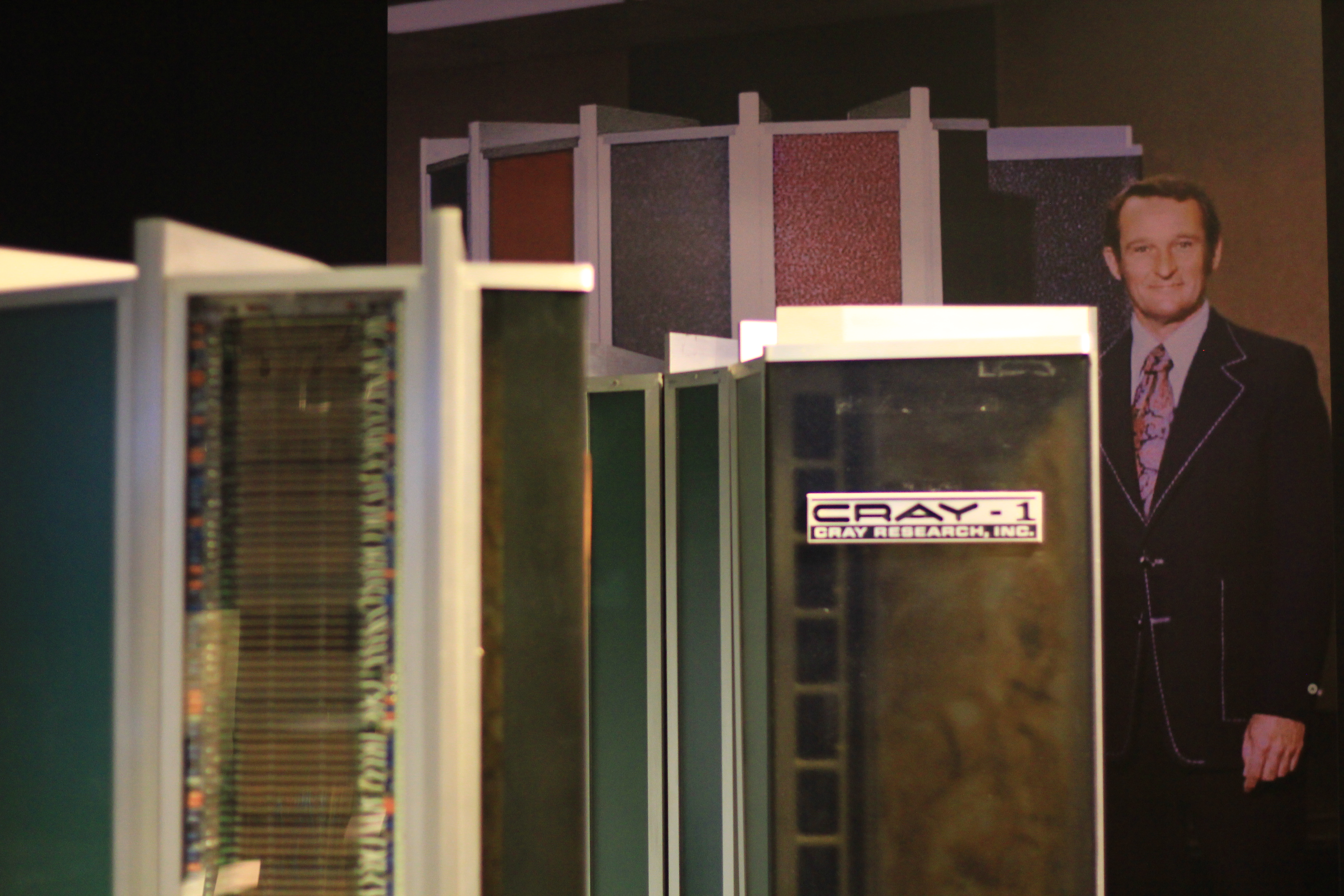
The vector supercomputer was the culmination of a design philosophy Seymour Cray had pursued since the 1960s. Scientific computing, Cray saw, spends most of its time doing the same arithmetic over and over on long lists of numbers – adding one array of a thousand numbers to another, multiplying a third. A conventional processor fetches, decodes and executes each of those thousand additions as a separate instruction. A vector processor treats the whole list as one object and streams it through a deeply pipelined arithmetic unit, so that once the pipeline is full it produces a result every clock tick. To make the clock tick fast enough to matter, Cray built his processors from the most aggressive logic available – emitter-coupled logic, later gallium arsenide – packed as densely as thermal engineering would allow and cooled by exotic means. The machines were beautiful and extreme. The Cray-1 of 1976 was a cylinder wrapped in a padded bench, its wiring hand-tuned so no signal path ran longer than it had to, the subject of Post 26.9 Its ancestors, the Control Data CDC 6600 and CDC 7600 that Cray designed in the 1960s, established the category “supercomputer” and are the subjects of Post 30 and Post 32.10
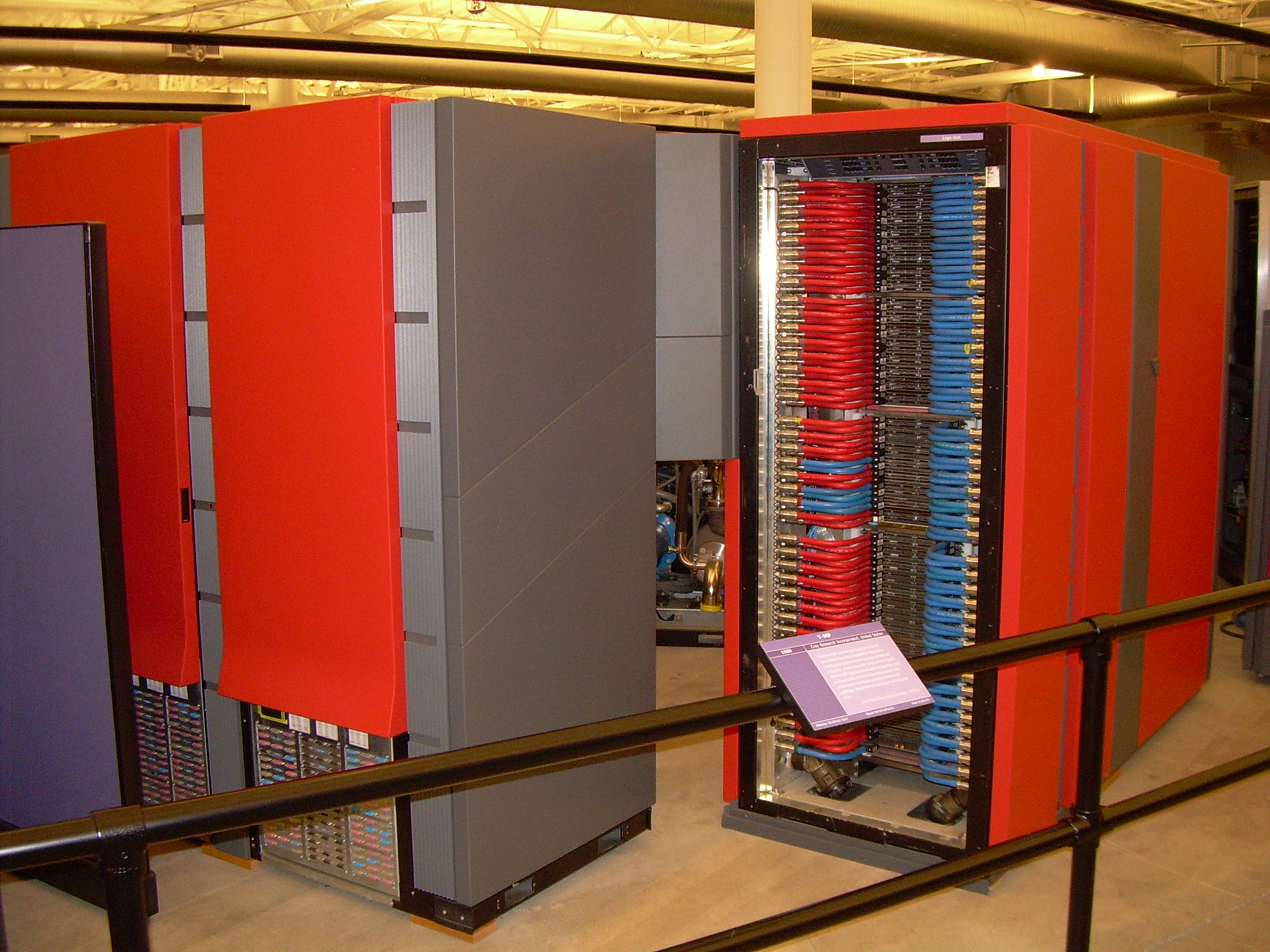
The defining property of these machines, for the argument that follows, lay in the memory rather than the vector pipeline. A Cray was a shared-memory machine. It had one large memory, and every processor in it – one in the Cray-1, up to sixteen in the C90 that crowned the line in 1992 – could see the whole of that memory directly, reaching any word of it with equal ease. When there was more than one processor, they cooperated by reading and writing the same shared variables, the way several people work on one whiteboard. For a programmer this was a gentle world. The forecast code was a single program; the compiler and a little hand-tuning arranged for the inner loops to vectorise and, later, for the outer loops to be shared across the handful of processors; the data all lived in one place and any part of the program could touch any part of it. Two decades of meteorological software – the spectral models, the grid-point models, the analysis schemes – had been written and tuned and re-tuned inside this world. When the European Centre for Medium-Range Weather Forecasts installed its Cray C90 in 1992, it was running a machine its scientists understood in their bones, the latest and grandest expression of an architecture their whole discipline had grown up on.11
The economics of that world were the economics of a monopoly on excellence. Only a few customers on Earth could ever afford the top of the vector line – the weather centres, the nuclear-weapons laboratories, a few oil companies and aerospace firms, a handful of national computing services. A high-end machine cost tens of millions of dollars, and its custom processors were designed, fabricated and assembled in tiny quantities for exactly this handful of buyers. The whole business rested on selling a small number of extraordinarily expensive machines to a small number of extraordinarily well-funded institutions. It was magnificent as long as no cheaper way existed to reach the same speed. The killer-micros thesis was, at bottom, the claim that a cheaper way was coming, and that when it arrived the economics of the custom vector processor would collapse from underneath. You cannot amortise the design of a bespoke processor across a dozen customers when your competitor amortises his across the entire computer industry.
2. The economics of the insurgency
The engine of the insurgency was the thing Gordon Moore had described in 1965 and the semiconductor industry had turned into a self-fulfilling prophecy: the steady exponential growth in the number of transistors on a chip of silicon, and with it the steady growth in the speed of the microprocessor. The microprocessor was a general-purpose computer on a single chip, and by the late 1980s a new generation of them – the reduced-instruction-set-computing, or RISC, chips – had reached an arithmetic performance that would have been the envy of a supercomputer a decade before. The Digital Equipment Corporation’s Alpha, the IBM POWER, the MIPS R-series, the Intel i860, the SPARC of Sun Microsystems: these were fast, and they were cheap, because each was made in enormous volume for the workstation and server markets, and the colossal cost of designing and fabricating them was spread across those markets rather than across a dozen supercomputer sales.
The killer-micros arithmetic followed from that difference in volume. A custom vector processor and a commodity microprocessor were both, in the end, transistors on silicon, and both improved as the fabrication technology improved. But the microprocessor improved on the industry’s schedule, doubling roughly every couple of years because the whole industry was pushing it, while the custom vector processor improved only as fast as a tiny specialist company with a dozen customers could afford to push it. Two exponential curves with different growth rates will cross, and Brooks’s graph simply showed where. After the crossing, the single fastest processor you could buy would be a commodity part, not a custom one – and you could buy a great many of them for the price of one vector machine. So buy hundreds, or thousands, and set them all to work on the same problem at once. This was the massively parallel processor, the MPP: a swarm of ordinary processors in place of one enormous custom one.1 Brooks was not only a prophet. Livermore backed the thesis with money and effort, mounting a Massively Parallel Computing Initiative to port real production codes – weapons physics, computational chemistry – onto the new machines, a deliberate early proof that serious scientific software could be made to live on a swarm of commodity chips rather than on a single custom processor.12
There was a catch, and the whole drama turned on it. The vector supercomputer’s shared memory did not scale to a swarm. You cannot wire a thousand processors to one memory and let them all reach any word of it at equal speed; the physics and the economics both forbid it. So the massively parallel machine gave up shared memory. Each of its processors – each node – had its own private memory, which only it could touch directly. The nodes were joined by a fast network, and when one node needed data that lived in another node’s memory, the two had to cooperate by explicitly sending a message across that network: one node packaged the data and sent it, the other received it. This was distributed memory, and it was far harder to program than the shared whiteboard of the Cray. The comfortable assumption that any part of the program could touch any part of the data was gone. Now the data was scattered across a thousand private memories, and any computation that needed data from more than one of them had to be written as an explicit choreography of sends and receives. The killer micros were cheaper and, in aggregate, faster. The price of that cheapness was that twenty years of shared-memory software, including every operational weather model in the world, would have to be torn apart and rebuilt.
The vector makers understood the threat and answered it, for a while, by building ever more extreme custom machines – exactly the trap the killer-micros thesis predicted for them. Seymour Cray left Cray Research in 1989 to found Cray Computer Corporation and chase the Cray-3, a machine whose processors were built from gallium arsenide rather than silicon, an exotic and difficult material chosen for raw speed. Exactly one Cray-3 was ever delivered, to the National Center for Atmospheric Research in May 1993, and even that was a loan, not a sale. The company never found a paying customer, because by 1993 the massively parallel machines had reached a price and performance the gallium-arsenide monster could not touch. The Cray-4 that was to follow never shipped. When the company could not raise the last twenty million dollars or so to finish it, it filed for bankruptcy in March 1995.45 The most brilliant custom-vector machine ever designed had been beaten not by a better custom-vector machine but by a heap of ordinary chips.
3. The new machines
The massively parallel machines came from several directions at once, and for a few years in the early 1990s the field was a riot of competing architectures, each betting on a different commodity processor and a different way of wiring the swarm together.
The most flamboyant came from Thinking Machines Corporation, a Cambridge, Massachusetts startup founded on the doctoral ideas of Danny Hillis. Its Connection Machine CM-2, delivered from 1987, was a machine of the purest parallel faith: up to sixty-five thousand five hundred and thirty-six tiny one-bit processors, arranged in a hypercube, all executing the same instruction at the same instant on their own separate scraps of data – a design called SIMD, for single instruction, multiple data. The CM-2 lived in a black cube studded with panels of blinking red lights, one of the few supercomputers ever built to be, deliberately, beautiful. But pure SIMD was rigid, and in 1991 Thinking Machines pivoted hard with the CM-5, dropping the hypercube of one-bit processors for a “fat tree” of commodity SPARC microprocessors, each a full independent computer running its own instructions – the design called MIMD, for multiple instruction, multiple data, which is the design essentially every parallel machine since has used.13
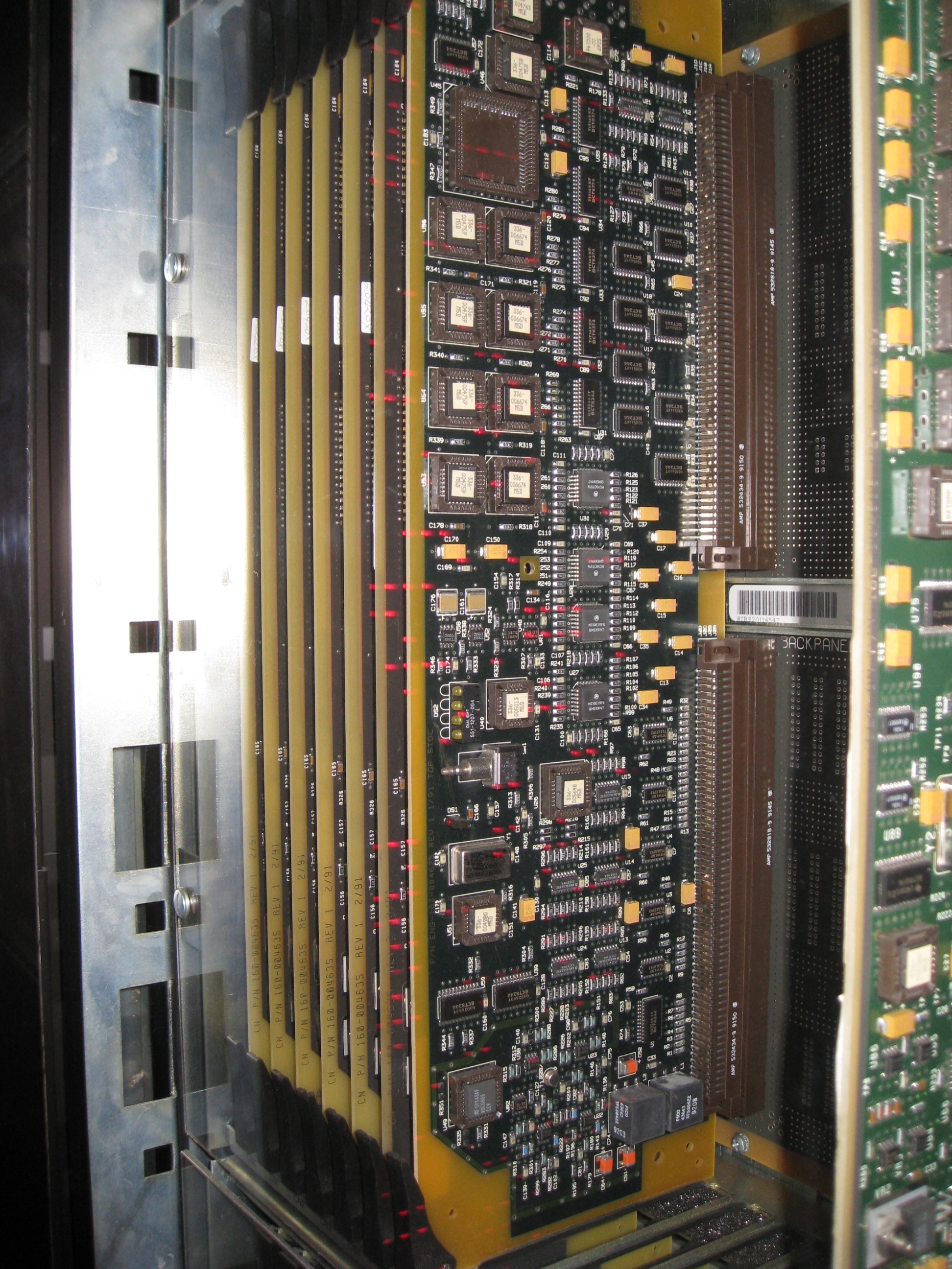
From Intel came the Paragon, delivered from around 1992, which laid its nodes out in a flat two-dimensional mesh, like a grid of tiles, and put two Intel i860 microprocessors in each node – one to compute, one to handle the traffic of messages crossing the mesh.14 From IBM came the RS/6000 SP, introduced as the SP1 in February 1993 and the SP2 in 1994, which took the same POWER microprocessors IBM sold in its ordinary workstations and joined them with a proprietary high-performance switch. The SP line was one of the most commercially successful of the early MPPs, and one of its descendants, Deep Blue, beat Garry Kasparov at chess.15 The architect of the SP’s scalable design at IBM was Marc Snir, who had taken his mathematics doctorate at the Hebrew University of Jerusalem in 1979 and who would, in one of the reversals this story keeps throwing up, receive the IEEE Seymour Cray Award in 2013.16
These were only the largest combatants. There were others – the nCUBE hypercubes, one of which had carried Gustafson’s thousandfold speed-up; the Meiko Computing Surface out of Bristol, built first on the transputer and later on commodity processors; a scattering of academic and startup machines that flared and died. For a few years no one could say with confidence which processor or which network topology would prevail, and buying a massively parallel machine meant betting on a design that might be orphaned within the decade. That uncertainty was itself the strongest possible argument for a portable software standard: portability was the only insurance a customer could buy against betting on the wrong horse.
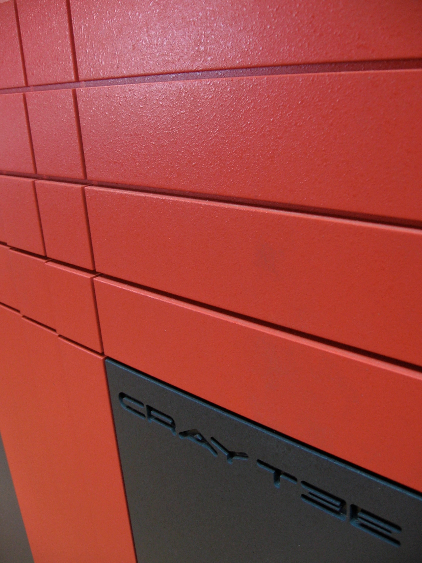
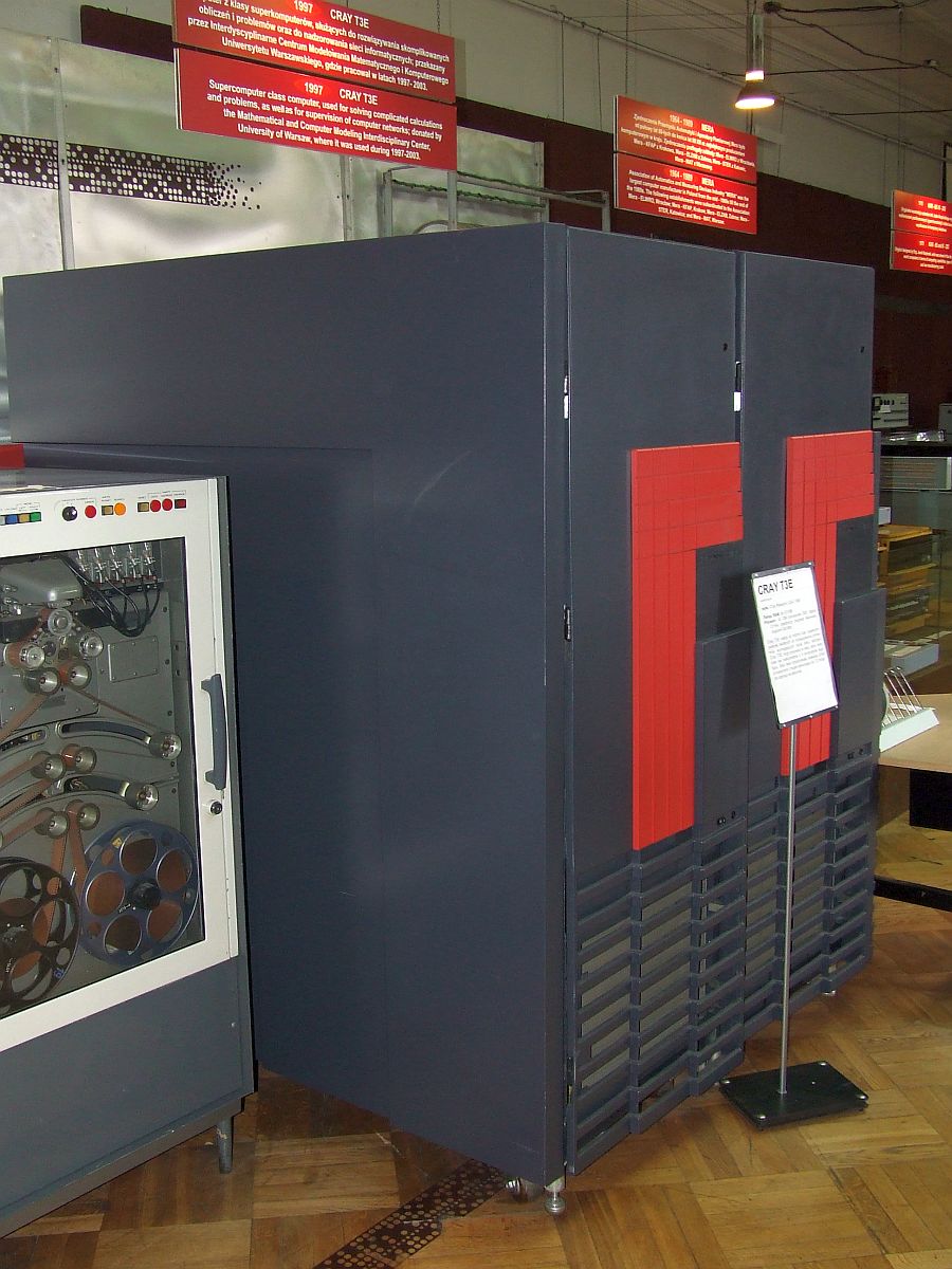
And then, most poignantly, the massively parallel machine came from Cray Research itself – the profitable parent Seymour Cray had left behind, not his breakaway company, which read the writing on the wall and built an MPP of its own. The Cray T3D, launched on 27 September 1993, was the first Cray machine ever built around another company’s processor: the Digital Alpha 21064, a commodity RISC microprocessor, hundreds or thousands of them wired into a three-dimensional torus, the doughnut-shaped network that gave the machine its name.17 The T3D still needed a conventional Cray vector machine bolted to its side as a “front end”, feeding it work and handling its input and output – a hybrid that betrayed how new and strange the MPP world still was to a vector company. Its successor, the Cray T3E, launched in late 1995, cut that cord. It was a fully self-hosting massively parallel machine, built around the faster Alpha 21164, needing no vector front end at all.18 The T3E was a landmark. In 1998 a 1480-processor T3E became the first supercomputer anywhere to sustain more than a trillion floating-point operations per second – one teraflop – on a real scientific application rather than a benchmark.18 The company Seymour Cray had built crossed over to the enemy’s architecture, and thrived there for a time.
The scoreboard for all this appeared in June 1993, and it made the transition visible and quantitative for the first time. Four computer scientists – Hans Meuer and Erich Strohmaier of the University of Mannheim, Jack Dongarra of the University of Tennessee, and Horst Simon – began publishing, twice a year, a ranked list of the five hundred most powerful computers on Earth, measured by their speed on a standard dense-linear-algebra benchmark called Linpack. They called it the TOP500.19 The very first list told the story at a glance: at its summit sat a Thinking Machines CM-5, in a 1024-processor configuration at the Los Alamos National Laboratory, sustaining 59.70 gigaflops – billions of floating-point operations per second – with no Cray vector machine anywhere near the top.2021 Vector supercomputers were still plentiful on that first list, but they were being pushed down it, and over the next few years anyone could watch, list by list, the massively parallel machines climb and the vector machines sink.
4. Amdahl against Gustafson
Before any of these machines could be taken seriously, a piece of received wisdom had to be overturned – a theoretical objection that had hung over massive parallelism for twenty years and told you, with the authority of simple algebra, that buying a thousand processors was a fool’s errand.
Think of it as the problem of the dinner party. You are cooking a large meal. Most of the work – chopping, peeling, stirring a dozen pots – can be split among as many cooks as fit in the kitchen, but one dish, a delicate sauce, must be made by a single chef and cannot be hurried or divided. If the sauce takes an hour and everything else takes nine hours for one cook, then one cook finishes in ten hours. Add cooks and the nine hours of divisible work shrinks – two cooks do it in four and a half, ten cooks in a bit under one – but the sauce still takes its stubborn hour. With an infinite brigade the divisible work vanishes and the meal still takes an hour, the length of the sauce. No matter how many cooks you hire, you can never finish in less than an hour, because a fixed fraction of the job is irreducibly serial. That floor, set by the un-parallelisable part, is the whole objection.
Its formal statement is Amdahl’s law, named for the computer architect Gene Amdahl, who put it forward in 1967. If a fraction s of a computation must be done serially – one step after another, on a single processor – and the rest can be spread perfectly across P processors, then the whole thing on P processors runs in time proportional to s + (1 - s) / P, and the speed-up over a single processor is 1 / ( s + (1 - s) / P ). Let P grow without limit and the speed-up climbs only to 1 / s. If just five per cent of your work is serial, then s = 0.05 and your maximum speed-up is 1 / 0.05 = 20 – twentyfold, and no more, though you buy a million processors.22 For a machine meant to carry a thousand processors, a ceiling of twenty was a death sentence. Amdahl’s law was the standard reason serious people gave, all through the 1970s and 1980s, for not believing in massive parallelism.
The reframing that broke the objection came from John Gustafson, then at Sandia National Laboratories, in a two-page note in the Communications of the ACM in May 1988, drily titled “Reevaluating Amdahl’s Law”.2324 Gustafson had just done what Amdahl’s law said was pointless. On a 1024-processor nCUBE hypercube at Sandia, he and his colleagues ran three real scientific applications and measured speed-ups of 1021, 1020 and 1016 – very nearly the full 1024, as if the serial fraction had barely existed.24 How could a machine reach a thousandfold speed-up when the algebra forbade more than a small multiple?
Amdahl had asked the wrong question. His law fixes the size of the problem and asks how much faster many processors solve that same fixed problem. But that is not what anyone does with a bigger machine. Nobody buys a thousand-processor computer to solve yesterday’s problem faster; they buy it to solve a bigger problem in the same time. Back to the kitchen. You do not use a hundred cooks to make the same ten-hour meal in a few minutes. You use a hundred cooks to cater a banquet a hundred times larger, in the same evening – and the sauce still takes its one hour, but that hour is now a trivial slice of a vastly larger job, so the brigade runs at nearly full efficiency. As the problem grows with the machine, the serial part stays roughly the same size while the parallel part swells, and the serial fraction shrinks toward nothing. Under this “scaled” or “weak” scaling, the speed-up on P processors is no longer capped at 1 / s; it grows very nearly in proportion to P itself – roughly P minus a small correction for the serial part.22 The two laws do not contradict each other. They are the same algebra under two different assumptions about whether the problem stays fixed or grows with the machine. Gustafson’s shift was one of perspective, and it was decisive: it turned the case for massive parallelism from absurd into obvious.22
And it was, above all, the natural case for numerical weather prediction. A weather centre has never wanted yesterday’s forecast computed faster. It has always wanted a better forecast – a finer grid, more vertical levels, more physics, more ensemble members – delivered inside the same immovable operational window of a few hours between the arrival of the observations and the moment the forecast must go out. That is weak scaling exactly: grow the problem with the machine, hold the wall-clock time fixed. Gustafson’s law was the permission slip that made it rational for a forecasting centre to buy a thousand processors, because the thing it wanted to do with them was precisely the thing a thousand processors excel at. The refinement of resolution this series traced through the spectral models of Post 39 was, from the hardware’s point of view, an engine for consuming parallelism.25
5. The Babel
Gustafson’s law said the swarm was worth harnessing. It did not say how, and the how was, for several years, a nightmare – because every one of the new machines spoke its own private language for the one operation that mattered most.
On a distributed-memory machine, recall, the whole game is the message: a computation that needs data from another node’s private memory can proceed only by an explicit exchange, one node sending and another receiving. Everything a programmer does on such a machine is built out of these sends and receives, so the library of message-passing operations is the foundation of the code. The trouble in the early 1990s was that there was no standard library. Each vendor supplied its own. Intel’s machines spoke a message-passing dialect called NX. Thinking Machines’ CM-5 spoke CMMD. IBM’s and nCUBE’s machines each had their own. Alongside the vendor dialects ran a scattering of portable-in-principle research libraries, each with its following: PVM, the Parallel Virtual Machine, written at Oak Ridge National Laboratory from 1989 and by far the most widely used, aimed at knitting networks of workstations into a single virtual machine; Express, from the company ParaSoft; p4 and Chameleon from Argonne; PARMACS from the German research world; Zipcode, built at Caltech on top of something called the Reactive Kernel.2627
PVM was, in an irony that recurs throughout this story, partly the work of the very people who would soon build the standard that superseded it. Jack Dongarra, one of PVM’s co-creators, became one of the central figures of the effort to replace it. The pre-standard world was not built by the careless. It was built by exactly the people clever enough to see that a thicket of private dialects had to give way to something common, and disciplined enough to make their own popular libraries obsolete to get there.
The consequence was a portability catastrophe. A forecast model, or any large scientific code, that had been painstakingly parallelised and tuned for an Intel Paragon, using Intel’s NX calls threaded through tens of thousands of lines, was dead weight on a Thinking Machines CM-5, which understood not a word of NX. To move it you had to find every message-passing call and rewrite it in the new machine’s dialect – and then, if you bought a third kind of machine three years later, do it all again. For a weather centre, which replaced its supercomputer every few years and had to protect an investment of hundreds of person-years in its model code, this was intolerable. The whole promise of the killer micros – cheap, abundant, ever-improving commodity hardware – was mortgaged to the fact that the software written for one generation could not survive the move to the next. The machines were a Babel, and until they could be made to speak a common tongue, the economic case for abandoning the comfortable vector monoculture was badly compromised. You would save money on the hardware and spend it all, and more, rewriting your software at every upgrade.
There was a real fear, voiced at the time, that message passing was simply too low-level and too machine-specific ever to be standardised – that parallel programming would stay a craft practised separately on each make of machine, the way assembly language had been. The Babel was not a temporary inconvenience. For a few years it was a genuine reason to doubt the killer micros could win at all.
6. The standard
The tower came down between 1992 and 1994, and it came down because a large, argumentative, mostly volunteer committee decided to bring it down.
A standard message-passing interface had been in the air since a small workshop in the summer of 1991, held at a mountain retreat in Austria, where a handful of researchers – Jack Dongarra, the German parallel-computing researcher Rolf Hempel, the British physicist-turned-computer-scientist Tony Hey, and David Walker of Oak Ridge – sketched a first white paper for a common interface, borrowing heavily from Marc Snir’s work at IBM.2628 The effort turned formal at a workshop on “Standards for Message Passing in a Distributed Memory Environment”, held at Williamsburg, Virginia, on 29 and 30 April 1992, organised by Dongarra and Walker.26 Out of Williamsburg came a working group, a name – MPI, the Message Passing Interface – and a preliminary draft, put forward at Supercomputing 1992 that November.2629 Through the first nine months of 1993 the working group, now the open-membership MPI Forum, met roughly every six weeks, and its draft was presented at Supercomputing 1993. After a period of public comment, the MPI-1.0 standard document, dated May 1994, was released that June.26
The remarkable thing about the MPI Forum was its breadth. Something like eighty people from around forty organisations took part – the hardware vendors whose incompatible dialects were the problem in the first place, the national laboratories, the universities, and a substantial European contingent alongside the Americans.26 The competitors sat in one room and agreed on a common language, because each had understood that a fragmented market served none of them, and that the customers – the weather centres and the weapons laboratories among them – were demanding portability as a condition of buying at all. The point-to-point communication group, which fixed the exact semantics of the fundamental send and receive, was led by Snir, Bill Gropp and Ewing Lusk; the minutes and much of the connective labour fell to Lusk; Dongarra, Walker, Hempel, Hey and Steve Otto, author of the Zipcode library, were all among the principals.263016 Between them, these were the people who had built the very dialects MPI was designed to replace. Rolf Hempel, in the German research world, had built PARMACS, a portable message-passing macro library, and carried that European experience into the standard.31 Steve Otto had built Zipcode.29 Tony Hey had come to parallel computing from particle physics, by way of Oxford, Caltech and CERN, and had pioneered distributed-memory message passing in the 1980s before co-writing the first MPI draft.32 Dongarra had co-built PVM, the most widely used pre-MPI system of all. They were, in effect, agreeing to obsolete their own creations in favour of a common one – exactly what a standard demands, and what makes real standards so rare. For the forecast centres watching from outside the committee room the stakes were concrete: a durable common interface was the only thing that would let a model code, representing hundreds of person-years of scientific labour, outlive the machine it was written for and cross intact into the next procurement. Jack Dongarra, born in Chicago in 1950, would receive the Turing Award, computing’s highest honour, in 2021, in part for this kind of standard-building work.30
What MPI standardised was a vocabulary, not a program: a precise, portable set of operations that every conforming machine had to provide, with identical meanings, callable from Fortran and C. It fixed the point-to-point operations, the send and receive between two named processes. It fixed the collective operations, in which a whole group of processes cooperate at once – a broadcast that sends one process’s data to all the others, a gather that collects a piece from every process onto one, a scatter that does the reverse, a reduction that sums or combines a value across all processes. It introduced the communicator, an object bundling a group of processes with a private communication context, so that messages sent inside one software module could never be confused with another’s – an abstraction that let large parallel programs be built out of independently written parallel libraries. And it introduced derived datatypes, a way to describe the scattered, strided chunks of an array that a real scientific code needs to move, so that the awkward geometry of a subdomain’s boundary could travel in a single well-described message. The forecast codes to come would lean on every one of these.
A standard on paper is worth nothing until someone proves it can be implemented, and implemented efficiently, on every machine. That was the work of MPICH, the reference implementation written by Gropp and Lusk at Argonne National Laboratory, with Mississippi State University, from 1992 onward, tracking the standard as it evolved. Its name encoded its lineage: MPI, plus CH for Chameleon, Gropp’s earlier portable library, on which it was built.33 MPICH was public-domain and portable, and it served two purposes at once. It proved the standard was implementable, and it handed every vendor and every laboratory a working MPI on day one, which many vendors took as the basis for their own optimised versions. Gropp and Lusk documented the effort in a 1997 paper with the agricultural title “Sowing MPICH”.34 Ewing Lusk – “Rusty” to everyone – had come to computing from pure mathematics, with a doctorate from the University of Maryland in 1970, and had joined Argonne in 1982; Bill Gropp would later direct the National Center for Supercomputing Applications.35 MPI-2 followed in 1997, adding parallel input and output, one-sided communication and dynamic process management, but the essential victory was already won with MPI-1. The Babel had a common tongue, and a code written against it would run on the Intel machine, the IBM machine, the Cray machine and the next machine, unchanged.26
Here is the deeper pattern, and it is the same one that ran through the previous post. Post 48 told how satellites finally let the Southern Hemisphere forecast catch up, and insisted that the enabling machine of that revolution was not a satellite or a supercomputer but a piece of software – the fast radiative-transfer model that let raw radiances be assimilated at all.36 The killer-micros revolution has the same shape. The commodity microprocessor was necessary but not sufficient; the machines it made possible were unusable, a Babel of incompatible dialects, until a piece of software – MPI – turned them into a coherent target a durable, portable, long-lived scientific code could be written against. The hardware got the headlines and the TOP500 rankings. The software is what actually let the weather models move.
7. Tiling the globe
To see what “moving the weather model” meant, look at the programming model MPI enabled, the one on which essentially every parallel forecast code has been built since. It is called domain decomposition, and its central idea needs no equation.
A forecast model works on a representation of the atmosphere spread over the surface of the globe and up through its depth – in the simplest picture, a grid of points blanketing the Earth, each point holding the temperature, pressure, wind and humidity of a little parcel of air, the whole thing stepped forward in time in small increments. On a shared-memory vector machine that grid lived in one memory and the single program marched it forward. On a distributed-memory machine with a thousand private memories, the grid has to be cut up and parcelled out. So you take the map of the globe and you tile it: you divide it into rectangular patches and hand one patch to each processor, which stores in its own private memory only the parcels of air inside its patch and is responsible only for stepping those forward. That is domain decomposition – splitting the map of the globe into tiles, one to a processor, so that a thousand processors work on a thousand different parts of the atmosphere at once.
The difficulty, and the reason MPI’s messages are needed, lives at the edges of the tiles. To step a grid point forward, a weather model needs to know what the atmosphere is doing at the neighbouring points – winds converge, pressure gradients push, the value at each point at the next instant depends on the values around it now. For a point deep in the interior of a processor’s tile, all the neighbours are in the same tile, in the same private memory, ready to hand. But for a point on the very edge of a tile, some neighbours lie across the border, in the tile belonging to the processor next door, in a different private memory this processor cannot touch. So before each step, every processor must obtain a copy of the thin strip of data just outside its own borders – the values along the edges of its neighbours’ tiles. That strip is the halo, or the ghost zone: a one- or two-cell-deep border, copied from the neighbour, that surrounds each tile and supplies the off-tile neighbour values the edge points need. And obtaining it is exactly a message. Each processor sends the data along its borders to its neighbours and receives, in return, their border data to fill its own halo. This is halo exchange, the heartbeat of a parallel grid-point model – a burst of neighbour-to-neighbour messages before every time step, filling the halos, after which every processor marches its own tile forward independently until the next step.
The virtue of halo exchange, from the point of view of a machine with a thousand processors, is that it is local. Each processor talks only to its handful of immediate neighbours, sending only the thin data along its shared borders. Make the machine bigger and the tiles smaller, and the interior work on each tile shrinks with the tile’s area while the halo traffic shrinks with the tile’s perimeter – and area falls faster than perimeter, so the communication stays a manageable fraction of the whole. Add more processors, give each a smaller tile, and the halo exchange does not choke; the neighbours are still just neighbours. This is exactly the weak scaling Gustafson had described, made concrete in the geometry of a weather grid. A grid-point model, decomposed into tiles and stitched together by halo exchange, is close to an ideal citizen of the massively parallel world. The trouble, for the leading forecast centres, was that their flagship models were not grid-point models. They were spectral models, and the spectral method does not decompose into local tiles.
8. The weather code’s reckoning
Moving the operational forecast models from the vector supercomputer to the massively parallel machine was, for the weather centres, a project of years and of wrenching re-engineering. It is easy, from a distance, to call it “porting the code”, as though it were a matter of recompiling. It was nothing of the sort. It was the reconstruction of software that in some cases embodied two decades of accumulated scientific labour, rebuilt around an assumption – distributed memory, explicit messages – that its original authors had never had to make.
The gentler case, and the instructive one to take first, was the British Meteorological Office’s Unified Model. It was a grid-point model – the same model family used for both weather forecasting and climate simulation, hence “unified” – and being a grid-point model it decomposed, as we have just seen, into tiles joined by halo exchange, the friendly case. The Met Office moved it from its shared-memory Cray vector machines onto the Cray T3E in the second half of the 1990s; version 4.2 was the first release able to run on the T3E, giving the model distributed-memory capability with no change to the underlying science.37 The parallel Unified Model used message passing for portability – MPI, and on the Cray hardware also Cray’s own low-latency SHMEM library – to perform the neighbour-to-neighbour halo swaps around each processor’s tile.3738 There was even a subtlety of arithmetic to attend to. The old Cray vector machines used Cray’s proprietary floating-point format, while the T3E, built around a commodity DEC Alpha, used the industry-standard IEEE format, which offered more precision but a smaller range, so the migration came with conversion utilities and a careful audit of the numerics.37 This was the Met Office at Bracknell, the same institution whose Cyber 205 struggles of the previous decade were the subject of Post 42; a decade on, it was moving its flagship model onto a machine built from commodity Alpha chips.8
The European Centre’s path was more complicated, because it was managed as a deliberate, staged retreat from shared-memory vector toward distributed-memory parallelism rather than a single leap, and because its flagship model was spectral. The Centre’s machine lineage tells the story in hardware. It ran the shared-memory vector Cray line to its summit, the sixteen-processor Cray C90 of 1992. Then, in September 1996, it took its first step into distributed memory with the Fujitsu VPP700 – a fascinating hybrid, a transitional machine that was parallel-vector. Its many processing elements were each still a fast vector processor in the Cray tradition, but they had private memories and communicated by messages, distributed-memory style.11 The VPP700 at Reading had forty-six processing elements, thirty-nine of them devoted to computation.11 This series has met it before: the VPP700 was the very machine on which four-dimensional variational assimilation, the subject of Post 47, went operational in November 1997.39 The parallel-vector Fujitsus were a bridge – vector processors, to keep the old vectorised code running fast, but wired together the distributed-memory way, to force the software toward message passing. The Centre followed the VPP700 with the more powerful VPP5000 around 2000, and then, in 2002 and 2003, made the full crossing to a scalar massively parallel machine of exactly the killer-micros kind: an IBM cluster of some fourteen hundred POWER4 processors – the same commodity family IBM sold in its commercial servers – described by the Centre as its first massively parallel system, followed by an enhanced POWER4 cluster in 2004.1140
Making the Integrated Forecasting System – the IFS, the Centre’s spectral model – run across those distributed processors was the labour of a dedicated parallelisation effort through the mid-1990s, documented in a 1995 paper in Parallel Computing with the plain title “The IFS model: a parallel production weather code”, by Saulo Barros, David Dent, Lars Isaksen, G. Robinson, George Mozdzynski and F. Wollenweber.41 Mozdzynski in particular would remain, for the next two decades, the figure most associated with the hard problem of making the IFS scale.4142 The IFS was parallelised for distributed memory with MPI for the message passing between processors, and later with OpenMP directives for the shared-memory parallelism within each multi-processor node – a hybrid style that recognised the machines themselves had become hybrids, clusters of shared-memory nodes.38 None of this was a recompilation. The IFS of the mid-1990s was a large body of Fortran, accreted over years and tuned in every inner loop to the shared-memory vector machine; making it run correctly and efficiently across dozens and then hundreds of private memories meant rethinking how every field was laid out, how every global operation was performed, and how the work was balanced so no processor sat idle while its neighbours laboured. It was effort measured in person-years, carried out by small teams under the same immovable deadline that governed everything at a forecasting centre: the new code had to produce, every single day, a forecast at least as good as the old one, on time, or it could not be deployed at all. Overseeing the Centre’s computing through these transitions was Geerd-Rüdiger Hoffmann, who led ECMWF’s computing side and who, tellingly, organised and edited the Centre’s series of workshops on “The Use of Parallel Processors in Meteorology” – the recurring gathering, running through the early and mid-1990s, at which the whole discipline hashed out precisely this migration, and whose proceedings Hoffmann collected under the title The Dawn of Massively Parallel Processing in Meteorology.43 The very existence of that workshop series, and that title, measures how consuming the transition was: an entire field convening, again and again, to work out how to survive the killer micros.
9. The spectral irony
Here the story reaches its sharpest point, an irony that sits at the exact intersection of the two threads this series has followed – the mathematics of the forecast and the machines that compute it.
The spectral transform method was the great methodological victory of numerical weather prediction in the 1970s and 1980s, the subject of Post 39.25 Rather than represent the atmosphere only as values on a grid of points, the spectral method represents the smooth global fields – and in particular their horizontal derivatives, which the equations of motion need at every step – as sums of waves wrapped around the sphere, the spherical harmonics, the natural musical notes of a globe. Computing derivatives, clumsy and inaccurate on a grid, becomes exact and trivial in this wave representation, which is why the method won: on the vector supercomputers of its era it delivered more accuracy per unit of computation than any grid-point scheme, and it swept the field’s leading global models. The reason it won is precisely the reason it would suffer on the massively parallel machine. The spherical harmonics are global. Each wave is spread over the entire sphere, so the transformation between the grid representation and the wave representation mixes together data from all around the world. And global mixing is the mortal enemy of the tile-and-halo model that makes a grid-point code scale.
Follow the data through one time step and the problem turns concrete. The physics of the atmosphere – the sunlight, the condensation, the friction – is computed on the grid, in physical space, where each processor could happily own a tile. But the dynamics wants the wave representation, and getting there takes two transforms in succession: first a Fourier transform along each line of latitude, turning the values around a latitude circle into east-west waves, then a Legendre transform down each line of longitude, combining those into the spherical harmonics. The catch is that a Fourier transform along a latitude circle needs all the points on that circle present together, on one processor; and the Legendre transform that follows needs all the points down a meridian together, on one processor. No single fixed tiling of the globe can put both a whole latitude circle and a whole meridian on one processor at once. So the data cannot stay still. Between each stage it must be completely rearranged across the machine – gathered up and redealt so that whatever direction the next transform runs along is the direction now resident, in full, on each processor.4445
That rearrangement is the transposition strategy, and it is what the IFS uses. Rather than computing each transform in place with communication tangled inside it, the IFS holds its data in a succession of four different layouts through each time step and moves between them by three wholesale redistributions – transposes.38 It begins in grid-point space, decomposed so each processor holds whole vertical columns over a patch of the globe. It transposes so that entire latitude circles come to rest on single processors, and does the Fourier transforms locally. It transposes again so the data the Legendre transform needs is resident, and does those locally. A final transpose brings it into full spectral space. Each transform, in this scheme, is purely local and needs no communication at all; all of the communication is concentrated into the transposes between them.38 The advantage is that the transforms run at full speed. The price is the nature of those transposes: they are all-to-all communications, in which every processor must send a piece of its data to every other processor at once. This is the costliest communication pattern there is, the opposite of the cheap neighbour-to-neighbour halo swap of a grid-point model. Halo exchange is a quiet word with the processor next door. An all-to-all transpose is every processor in the machine shouting to every other one simultaneously, and it stresses the machine’s network as nothing else does.44
There had been a genuine debate over how best to do it. One school – the distributed-transform approach – kept the data more or less in place and parallelised the transforms themselves, paying the communication cost inside each transform. The other – the transposition strategy – moved the data instead and kept every transform local. The two were compared carefully in the early 1990s by Saulo Barros and Tuomo Kauranne, and by Ian Foster and Patrick Worley, and for the global models of the leading centres the transposition strategy generally prevailed, because concentrating the communication into a few large, well-structured all-to-all exchanges used the network more efficiently than scattering it through the arithmetic.4445 But winning that internal argument changed nothing about the external fact. However you organised it, a global spectral transform demanded global communication, and global communication is the one thing a massively parallel machine does worst.
So the reversal was complete. The spectral method won the 1980s because it was the most efficient way to compute a global forecast on a vector supercomputer with a few shared-memory processors. On the massively parallel machine of the 1990s, that same global character turned it into the hardest thing to scale in all of numerical weather prediction – the one major method whose fundamental operation demanded the most expensive communication pattern a distributed-memory machine can perform, while the older, humbler grid-point models needed only the cheap and friendly halo swap. The method that had beaten the grid-point models on the old hardware was, on the new hardware, hobbled by exactly the property that had made it win.
The centres fought the scaling problem on several fronts and, for a long time, won. The reduced Gaussian grid – an arrangement that thins out the grid points along the latitude circles as they shrink toward the poles, so the points stay roughly evenly spaced on the ground rather than crowding at high latitudes – cut both the arithmetic and the volume of data that had to be transposed, and let the processors’ tiles be balanced so each held nearly the same number of points and none sat idle.4638 The transposes were tuned to the network; the message-passing used MPI’s all-to-all collective operation, the very operation the MPI Forum had standardised for exactly this kind of global rearrangement.38 And the raw performance climbed, spectacularly, decade over decade. By 1998 the IFS sustained around 100 gigaflops on a 1024-processor Cray T3E at its operational resolution of the day; by 2004, on the enhanced IBM POWER cluster, a much higher-resolution IFS reached one teraflop on two thousand and forty-eight processors.38 Later still, the all-to-all cost of the Legendre transform was attacked at its mathematical root, with a fast spherical-harmonics transform devised by Nils Wedi, Mats Hamrud and George Mozdzynski, which slowed the growth of that cost and kept the spectral method viable at resolutions approaching a couple of kilometres.42
But the deeper lesson was lost on no one, and it points past the end of this story. The all-to-all transpose cost of a global spectral model grows worse than the local halo cost of a grid-point model as the processor count climbs into the many thousands and beyond. That structural disadvantage – the global communication built into the heart of the spectral method – is what turned attention, in the research of the 2010s, back toward grid-point formulations, and toward finite-volume and icosahedral dynamical cores built on grids that need only local, neighbour-to-neighbour communication, the pattern the massively parallel machine rewards.47 The method the killer micros had wounded was still standing, patched and optimised, running the world’s leading forecasts. But the wound was real, and the search for a successor the swarm of processors would treat more kindly had begun. The hardware had reached back into the mathematics and changed which methods the field would pursue.
10. The aftermath
Brooks’s prophecy can be dated with unusual precision, because the industry it destroyed died on a public schedule.
The first to fall was ETA Systems, the Control Data spinoff that had built the ETA-10 and carried Control Data’s last hopes in the supercomputer business; Control Data shut it down in 1989, a first tremor that ties back to the Cyber 205 chapter of Post 42.8 Thinking Machines Corporation, the most visible of the massively parallel startups, was killed by the very revolution it had helped to start, not by the vector makers – undone by the end of generous defence funding, by recession, and by competition from the commodity-based machines that made its exotic hardware look expensive. It filed for Chapter 11 in August 1994; its hardware assets went to Sun Microsystems, and the shell re-emerged as a small parallel-software company.3 Cray Computer Corporation, Seymour Cray’s gallium-arsenide venture, filed in March 1995 without ever selling a machine.5 Cray Research, the profitable parent, was absorbed by Silicon Graphics for 740 million dollars in February 1996.6 And Seymour Cray himself died on 5 October 1996, of the injuries from the highway accident twelve days before.47 In about seven years the entire ecosystem of the custom vector supercomputer – the spinoffs, the startups, the founder’s own last company, and finally the founder – was gone or subsumed. The killer micros had done what the graph said they would.
What replaced them was, and remains, the architecture Brooks had described: large numbers of commodity microprocessors, in private-memory nodes, connected by a fast network and programmed by message passing. Every machine at the top of the TOP500 through the late 1990s and beyond was of this kind, and as the years passed even the line between a purpose-built massively parallel machine and a “cluster” of ordinary server nodes eroded, until the typical supercomputer became, frankly, a warehouse of rack-mounted commodity computers wired together. The killer micros had won so completely that the category of the exotic supercomputer all but dissolved into the mass market it grew from. The weather centres today run their forecasts on exactly such machines, tens or hundreds of thousands of commodity processor cores, their models threaded through with the MPI calls whose standardisation in 1994 made the whole edifice portable and durable.
The victory compounded on itself. Because the forecast models were now written in portable MPI against distributed memory, each new generation of cheaper and more numerous commodity processors could be absorbed without another ground-up rewrite; the software investment made once, in the painful decade of the 1990s, paid out across every procurement that followed. The resolution of the operational forecast climbed. The ensembles grew from tens of members toward hundreds. The reanalyses that reconstruct decades of past weather, which lean on running a modern assimilation system over archived observations, became feasible only because that assimilation could be spread across thousands of processors at once. The killer micros did not just win a contest of hardware. They set the terms on which every subsequent advance in the forecast would be bought.
For numerical weather prediction the transition was not just a change of hardware but a change of what the field’s software fundamentally was. The forecast model stopped being a single program marching a shared array forward and became a thousand copies of a program, each owning a tile of the world, cooperating by an incessant exchange of messages – halos swapped at the borders for the grid-point codes, whole hemispheres of data transposed across the machine for the spectral ones. The re-engineering consumed years of the best scientific-programming effort at every major centre, and it leaves little visible trace in the forecasts themselves, which simply kept improving. But it was the necessary passage. Without it, the models would have been marooned on a dying architecture; with it, they inherited the compounding cheapness of the commodity processor, and with that cheapness the resolution and the ensemble size and the richer physics the following decades delivered.
There is a final symmetry in it, of the kind history occasionally arranges without being asked. The custom vector supercomputer had been a monument to one idea: that the way to go fast was to build a single processor of surpassing excellence, whatever the cost, and to let a small elite of institutions pay for it. The killer micros embodied the opposite: that the way to go fast was to take the ordinary processor the whole world was already buying, and use a great many of them at once. The second idea won, comprehensively, on the economics Brooks had drawn as two crossing lines at a conference around 1990. Seymour Cray, who had spent his life perfecting the first idea, conceded the second in the end – his last company was to have built a massively parallel machine – and did not live to build it. He was killed in the autumn of 1996, in the same year the company bearing his name passed into other hands and the machines bearing his philosophy passed out of the world. The micros had attacked, as advertised. Nothing of the old order survived.
-
“Killer micro,” Wikipedia, https://en.wikipedia.org/wiki/Killer_micro. Eugene Brooks of the Lawrence Livermore National Laboratory coined “the attack of the killer micros,” a phrase fixed to his talk at Supercomputing 1990, though the idea was aired across roughly 1989-1990. The thesis: commodity microprocessors riding Moore’s-law economics, ganged in the hundreds and thousands, would overtake the custom vector CPU on price and performance. The full name “Eugene D. Brooks III” is widely repeated but not primary-confirmed, so only “Eugene Brooks” is asserted here. ↩ ↩2
-
The Jargon File (Eric S. Raymond, ed.), entry “killer micro,” at http://catb.org/~esr/jargon/html/K/killer-micro.html, corroborated by FOLDOC at https://foldoc.org/killer+micro. The catchphrase “nobody will survive the attack of the killer micros” is documented here as folklore attached to Brooks’s talk; it is a secondary attribution, not a verified verbatim primary quotation from Brooks, and is presented in the text as a catchphrase rather than a direct quote. ↩ ↩2
-
“Thinking Machines Corporation,” Wikipedia, https://en.wikipedia.org/wiki/Thinking_Machines_Corporation, with the Washington Post reorganisation story of 16 August 1994 at https://www.washingtonpost.com/archive/business/1994/08/16/thinking-machines-corp-to-file-for-reorganization/. Thinking Machines filed for Chapter 11 in August 1994; its hardware assets went to Sun Microsystems and the company re-emerged in 1996 as a small parallel-software firm. ↩ ↩2
-
“Seymour Cray,” Wikipedia, https://en.wikipedia.org/wiki/Seymour_Cray. Born 28 September 1925 in Chippewa Falls, Wisconsin; the accident (Jeep Cherokee, struck while merging onto Interstate 25 near the US Air Force Academy, rollover) is dated 23 September 1996; he died 5 October 1996, aged 71. Cray Computer Corporation filed Chapter 11 on 24 March 1995; the Cray-3 (gallium arsenide) had exactly one unit delivered, to NCAR in May 1993, and the Cray-4 never shipped. Cray founded SRC Computers in 1996, intending a massively parallel machine. ↩ ↩2 ↩3 ↩4 ↩5
-
Seattle Times, “Cray Computer Corp. files for bankruptcy protection,” 24 March 1995, https://archive.seattletimes.com/archive/19950324/2111923/cray-computer-corp-files-for-bankruptcy-protection; cray-history.net, “Cash-starved Cray Computer closes, seeks Chapter 11,” gives 27 March, at https://cray-history.net/2021/07/23/cash-starved-cray-computer-closes-seeks-chapter-11-march-27th-1995/. The filing date of 24 March 1995 is used, following the Seattle Times and the Seymour Cray Wikipedia record. ↩ ↩2 ↩3
-
“Cray,” Wikipedia, https://en.wikipedia.org/wiki/Cray, with the Washington Post, “Silicon Graphics to acquire Cray in 740 million deal,” 27 February 1996, at https://www.washingtonpost.com/archive/business/1996/02/27/silicon-graphics-to-acquire-cray-in-740-million-deal/. Silicon Graphics acquired Cray Research in February 1996 for 740 million dollars. ↩ ↩2
-
Washington Post, “Computer pioneer Seymour Cray dies,” 6 October 1996, https://www.washingtonpost.com/archive/local/1996/10/06/computer-pioneer-seymour-cray-dies/; HPCwire, “Seymour Cray dies,” 5 October 1996, https://www.hpcwire.com/1996/10/05/seymour-cray-dies/; Computer History Museum, this-day-in-history, https://www.computerhistory.org/tdih/october/5/. Cray died of head injuries sustained in the accident; his age at death was 71, though some contemporary wire copy erroneously said 70. ↩ ↩2
-
See Post 42, “The First in Bracknell”, on the Control Data Cyber 205 at the British Meteorological Office and its defeat by Cray in the vector-versus-vector procurement battles of the 1980s – a skirmish inside the vector family, as distinct from the death of the whole vector paradigm told here, and the chapter to which the shutdown of Control Data’s ETA Systems spinoff in 1989 traces back. ↩ ↩2 ↩3
-
See Post 26, “The Machine That Looked Like Furniture”, on the Cray-1 of 1976 – the cylindrical shared-memory vector supercomputer that defined the architecture numerical weather prediction ran on for two decades, and whose whole design philosophy the killer micros overturned. ↩
-
See Post 30, “Thirty-Four People, Including the Janitor”, on the Control Data CDC 6600, and Post 32, “Freon and Wire”, on the CDC 7600 – the two Seymour Cray machines of the 1960s that established the category of the supercomputer before he founded Cray Research. ↩
-
ECMWF, “The critical role of high-performance computing in medium-range weather forecasting: half a century of technology innovation,” https://www.ecmwf.int/sites/default/files/elibrary/81678-the-critical-role-of-highperformance-computing-in-medium-range-weather-forecasting-half-a-century-of-technology-innovation.pdf. The source for ECMWF’s machine timeline: the shared-memory vector Cray C90 (1992), the distributed-memory parallel-vector Fujitsu VPP700 operational from September 1996 (46 processing elements, 39 for computation), the Fujitsu VPP5000 around 2000, and the IBM POWER4 cluster of about 1400 processors described as ECMWF’s first massively parallel system (2002-2003), with an enhanced POWER4 cluster in 2004. ↩ ↩2 ↩3 ↩4
-
“Harnessing the killer micros: applications from LLNL’s massively parallel computing initiative,” Theoretical Chemistry Accounts (Springer), DOI 10.1007/BF01113270, https://link.springer.com/article/10.1007/BF01113270; an archived copy is at http://web.archive.org/web/20180609211940/https://link.springer.com/article/10.1007%2FBF01113270. Documents the Lawrence Livermore National Laboratory initiative, associated with Eugene Brooks’s killer-micros argument, to port production scientific codes onto massively parallel machines. ↩
-
“Connection Machine,” Wikipedia, https://en.wikipedia.org/wiki/Connection_Machine. The CM-2 (1987) was a SIMD hypercube of up to 65536 one-bit processors; the CM-5 (1991) pivoted to a MIMD fat-tree of commodity SPARC microprocessors. Danny Hillis’s doctoral work underlay the Connection Machine design. ↩
-
Netlib / University of Tennessee, “Advanced computers” notes on the Intel Paragon, https://www.netlib.org/utk/papers/advanced-computers.0/paragon.html. The Intel Paragon (from around 1992) arranged its nodes in a two-dimensional mesh with wormhole routing, each node carrying two Intel i860 XP microprocessors (one for computation, one for communication); the XP/S-150 at Oak Ridge National Laboratory was a large installation of this line. ↩
-
“IBM RS/6000 SP,” Wikipedia, https://en.wikipedia.org/wiki/IBM_RS/6000_SP, with the Netlib notes on the IBM SP2 at https://www.netlib.org/utk/papers/advanced-computers.0/sp2.html. The IBM RS/6000 SP appeared as the SP1 in February 1993 and the SP2 in 1994, built from commodity POWER microprocessors linked by IBM’s proprietary High-Performance Switch; a later member of the line, Deep Blue, defeated Garry Kasparov in 1997. ↩
-
Marc Snir, University of Illinois faculty page, https://siebelschool.illinois.edu/about/people/all-faculty/snir, with the SC13 announcement of his 2013 IEEE Seymour Cray Award at http://sc13.supercomputing.org/content/parallel-computing-pioneer-marc-snir-receive-2013-ieee-seymour-cray-award-sc13.html. Snir took his mathematics doctorate at the Hebrew University of Jerusalem in 1979, led the Scalable Parallel Systems group behind the IBM SP at IBM’s T. J. Watson Research Center, and was a principal developer of MPI; his birth date is not established here and is omitted. ↩ ↩2
-
“Cray T3D,” Wikipedia, https://en.wikipedia.org/wiki/Cray_T3D. Introduced 27 September 1993, the T3D was Cray Research’s first MPP and the first Cray machine built around another company’s processor – the 150 MHz DEC Alpha 21064 – with 32 to 2048 processing elements in a three-dimensional torus, hosted by a Cray vector front-end machine. ↩
-
“Cray T3E,” Wikipedia, https://en.wikipedia.org/wiki/Cray_T3E. Launched in late November 1995, the T3E used the DEC Alpha 21164 and was a fully self-hosting MPP requiring no vector front-end; a 1480-processor T3E-1200 became, in 1998, the first supercomputer to sustain more than one teraflop on a real scientific application. ↩ ↩2
-
“TOP500,” Wikipedia, https://en.wikipedia.org/wiki/TOP500, with TOP500’s own 25-years retrospective at https://www.top500.org/25years/. The TOP500 list was created by Hans Meuer, Erich Strohmaier, Jack Dongarra and Horst Simon, first published in June 1993, and ranks machines by their sustained performance (Rmax) on the Linpack dense-linear-algebra benchmark. ↩
-
TOP500 list of June 1993, https://www.top500.org/lists/top500/1993/06/. The number-one machine on the first list was a Thinking Machines CM-5 with 1024 processors at Los Alamos National Laboratory, sustaining 59.70 gigaflops; the second-ranked machine reached 30.40 gigaflops. ↩
-
TOP500 system record, “CM-5, Los Alamos National Lab,” https://www.top500.org/resources/top-systems/cm-5-los-alamos-national-lab/. Confirms the CM-5/1024 configuration at Los Alamos as the first TOP500 number one. ↩
-
C. Shi (Temple University), “Reevaluating Amdahl’s Law and Gustafson’s Law,” teaching notes deriving both laws and the strong-versus-weak-scaling distinction, https://cis.temple.edu/~shi/wwwroot/shi/public_html/docs/amdahl/amdahl.html. The source for the Amdahl speed-up 1/(s + (1-s)/P) with its ceiling of 1/s (a 5 per-cent serial fraction capping speed-up at 20), for Gustafson’s scaled speed-up growing nearly linearly in P, and for the observation that the two laws are the same algebra under different assumptions about whether the problem size is fixed or grows with the machine. ↩ ↩2 ↩3
-
“Gustafson’s law,” Wikipedia, https://en.wikipedia.org/wiki/Gustafson%27s_law. Confirms the citation and the weak-scaling reframing; John Gustafson’s birth date is not established here and is omitted. ↩
-
Gustafson, J. L., 1988: “Reevaluating Amdahl’s Law,” Communications of the ACM 31(5), 532-533, DOI 10.1145/42411.42415, https://dl.acm.org/doi/10.1145/42411.42415; the ACM page returns a 403, and an archived copy is at http://web.archive.org/web/20250706112423/https://dl.acm.org/doi/10.1145/42411.42415. Written October 1987, co-signed with Edwin Barsis of Sandia. The empirical basis was a 1024-processor nCUBE hypercube at Sandia National Laboratories, on which three real applications reached measured speed-ups of 1021, 1020 and 1016. ↩ ↩2
-
See Post 39, “Thirty-eight Years on the Sphere”, on the spectral transform method – the representation of the global atmosphere as sums of spherical-harmonic waves, which won the 1970s and 1980s on vector supercomputers and, precisely because of its global character, became the hardest method to scale on the massively parallel machines of the 1990s. ↩ ↩2
-
“Message Passing Interface,” Wikipedia, https://en.wikipedia.org/wiki/Message_Passing_Interface. The source for the standardisation timeline: the 1991 Austrian retreat white paper, the Williamsburg workshop of 29-30 April 1992, the preliminary draft at Supercomputing 1992, the MPI-1.0 standard document dated May 1994 and released that June, and MPI-2 in 1997; for the Forum’s scale (about 80 people from 40 organisations); for the pre-MPI dialects (IBM, Intel and nCUBE vendor libraries, PVM, Express, p4, PARMACS); and for what MPI standardised (point-to-point and collective operations, communicators, derived datatypes, Fortran and C bindings). ↩ ↩2 ↩3 ↩4 ↩5 ↩6 ↩7 ↩8
-
“Parallel Virtual Machine,” Wikipedia, https://en.wikipedia.org/wiki/Parallel_Virtual_Machine. PVM was first written at Oak Ridge National Laboratory in 1989 (Al Geist, Vaidy Sunderam, Jack Dongarra and others), rewritten at the University of Tennessee, and was the dominant portable message-passing system before MPI. ↩
-
Dongarra, J., R. Hempel, A. J. G. Hey and D. W. Walker, 1993: “A Proposal for a User-Level, Message-Passing Interface in a Distributed Memory Environment,” Oak Ridge National Laboratory Technical Report ORNL/TM-12231, February 1993 – the seed document for the MPI Forum, at https://impact.ornl.gov/en/publications/mpi-a-standard-message-passing-interface/. This draft, drawing on Marc Snir’s IBM work and Rolf Hempel’s PARMACS experience, brought the early proposal into the Forum. ↩
-
Dongarra, J., S. Otto, M. Snir and D. Walker, 1993: “A Message-Passing Standard for MPP and Workstations,” Communications of the ACM, https://www.researchgate.net/publication/220421514_A_Message_Passing_Standard_for_MPP_and_Workstations. An early published statement of the MPI effort, naming several of the Forum principals; Steve Otto was the author of the Zipcode library. ↩ ↩2
-
“Jack Dongarra,” Wikipedia, https://en.wikipedia.org/wiki/Jack_Dongarra, with the ACM A. M. Turing Award citation at https://amturing.acm.org/award_winners/dongarra_3406337.cfm. Dongarra was born on 18 July 1950 in Chicago; he co-built EISPACK, LINPACK, BLAS, LAPACK, PVM, MPI and the TOP500, and received the 2021 Turing Award. ↩ ↩2
-
Rolf Hempel’s publication record on dblp, https://dblp.org/pid/76/235.html, and the Argonne notice on the PARMACS pioneers at https://www.anl.gov/article/pioneers-of-highperformance-computing-library-reunite. Hempel, a German parallel-computing researcher associated with GMD (and later the German Aerospace Center, DLR), built the PARMACS portable message-passing macro library and co-authored the 1993 ORNL MPI draft. His birth date is not established here and is omitted. ↩
-
“Tony Hey,” Wikipedia, https://en.wikipedia.org/wiki/Tony_Hey. Anthony J. G. Hey took a doctorate in particle physics at the University of Oxford and worked at Caltech and CERN before becoming a professor of computation at the University of Southampton in 1986; he was a pioneer of distributed-memory message passing in the 1980s and a co-author of the 1993 ORNL draft that seeded MPI. His birth date is not established here and is omitted, as is any unverified honour. ↩
-
“MPICH,” Wikipedia, https://en.wikipedia.org/wiki/MPICH. MPICH – the name combining MPI with the CH of Gropp’s earlier Chameleon library – was the reference implementation, developed from 1992 by William Gropp and Ewing Lusk at Argonne National Laboratory with Mississippi State University, and became the base for many vendor MPI implementations. ↩
-
Gropp, W., and E. Lusk, 1997: “Sowing MPICH: A Case Study in the Dissemination of a Portable Environment for Parallel Scientific Computing,” International Journal of Supercomputer Applications 11(2), 103-114, DOI 10.1177/109434209701100204, https://journals.sagepub.com/doi/10.1177/109434209701100204. Documents the design and dissemination of the MPICH reference implementation. ↩
-
Ewing (“Rusty”) Lusk, Argonne National Laboratory homepage, https://www.mcs.anl.gov/~lusk/, and the Argonne notice of his appointment as MCS Division Director at https://www.newswise.com/articles/lusk-named-director-of-mathematics-and-computer-science-division-at-argonne. Lusk took his mathematics Ph.D. at the University of Maryland in 1970 and joined Argonne in 1982; William Gropp later became Director of the National Center for Supercomputing Applications. Their birth dates are not established here and are omitted. ↩
-
See Post 48, “The Hemisphere That Caught Up”, whose recurring motif is that the enabling machine of a revolution can be software rather than silicon – there the fast radiative-transfer model that made direct radiance assimilation possible, here the MPI standard that made the massively parallel machines usable by a durable, portable forecast code. ↩
-
“Unified Model,” Wikipedia, https://en.wikipedia.org/wiki/Unified_Model, with the Met Office Unified Model User Guide at https://www.ukscience.org/_Media/UM_User_Guide.pdf. The Unified Model is a grid-point model parallelised for distributed memory by halo (boundary) exchange; version 4.2 was the first release able to run on the Cray T3E, and the move from Cray-proprietary to IEEE floating-point number format (more precision, smaller range) accompanied the migration, with conversion utilities provided. ↩ ↩2 ↩3
-
Salmond, D., 2004: “Computer Architectures and Aspects of NWP Models,” ECMWF, https://www.ecmwf.int/sites/default/files/elibrary/2004/12066-computer-architectures-and-aspects-nwp-models.pdf. The source for the IFS transposition strategy (data held in four layouts – grid-point, then two intermediate states, then spectral – with three all-to-all transposes between them, each transform computed locally), for the reduced-Gaussian-grid load balancing, for the MPI-plus-OpenMP hybrid parallelisation, for the wide-halo swaps of the grid-point Unified Model, and for the performance figures (IFS around 100 gigaflops on a 1024-processor Cray T3E in 1998; about one teraflop on a 2048-processor IBM POWER cluster at higher resolution in 2004). ↩ ↩2 ↩3 ↩4 ↩5 ↩6 ↩7
-
See Post 47, “Eleven Years from the Adjoint”, on the operational deployment of four-dimensional variational assimilation at ECMWF on 25 November 1997 – which ran on the Fujitsu VPP700, the transitional distributed-memory parallel-vector machine that also marks ECMWF’s first step off the shared-memory Cray vector line. ↩
-
ECMWF, IFS Documentation, Part II: Data Assimilation, https://www.ecmwf.int/sites/default/files/elibrary/2014/9202-part-ii-data-assimilation.pdf. Corroborates the C90-to-VPP700-to-VPP5000-to-IBM machine progression in the operational context of the assimilation and forecast system. ↩
-
Barros, S. R. M., D. Dent, L. Isaksen, G. Robinson, G. Mozdzynski and F. Wollenweber, 1995: “The IFS model: a parallel production weather code,” Parallel Computing 21(10), 1621-1638, DOI 10.1016/0167-8191(96)80002-0, https://www.sciencedirect.com/science/article/abs/pii/0167819196800020; an archived copy of the abstract is at http://web.archive.org/web/20240416105243/https://www.sciencedirect.com/science/article/abs/pii/0167819196800020. The paper documenting the message-passing parallelisation of ECMWF’s Integrated Forecasting System; George Mozdzynski is confirmed here as a member of the IFS parallelisation team. ↩ ↩2
-
Wedi, N. P., M. Hamrud and G. Mozdzynski, 2013: “A Fast Spherical Harmonics Transform for Global NWP and Climate Models,” Monthly Weather Review 141(10), 3450-3461, DOI 10.1175/MWR-D-13-00016.1, https://journals.ametsoc.org/view/journals/mwre/141/10/mwr-d-13-00016.1.xml. A fast Legendre/spherical-harmonics transform that slowed the growth of the transform cost and helped keep the spectral method viable at very high resolution; George Mozdzynski is a co-author. ↩ ↩2
-
Geerd-R. Hoffmann’s publication record on dblp, https://dblp.org/pid/67/1818.html, and his edited volume The Dawn of Massively Parallel Processing in Meteorology (Springer), the proceedings of the ECMWF “Workshop on the Use of Parallel Processors in Meteorology,” listed at https://www.goodreads.com/author/show/2822679.Geerd_R_Hoffmann. Hoffmann led ECMWF’s computing side and organised and edited the Centre’s parallel-processing workshop series through the early and mid-1990s; the exact formal job title and tenure are not primary-confirmed and are hedged in the text, and his birth date is omitted. ↩
-
Barros, S. R. M., and T. Kauranne, 1994: “On the parallelization of global spectral weather models,” Parallel Computing 20(9), 1335-1356, https://www.sciencedirect.com/science/article/abs/pii/0167819194900418; an archived copy of the abstract is at http://web.archive.org/web/20240420162150/https://www.sciencedirect.com/science/article/abs/pii/0167819194900418. The canonical comparison of one- and two-dimensional static domain decomposition against the transposition strategy for spectral models, demonstrated on an Intel iPSC/2 hypercube; the transposition strategy redistributes the data between time-step stages so that every Fourier and Legendre transform is computed locally, concentrating all communication into all-to-all transposes. ↩ ↩2 ↩3
-
Foster, I., and P. H. Worley, 1997: “Parallel Algorithms for the Spectral Transform Method,” SIAM Journal on Scientific Computing 18(3), 806-837, DOI 10.1137/S1064827594266891, https://epubs.siam.org/doi/10.1137/S1064827594266891; an archived copy is at http://web.archive.org/web/20230308121751/http://epubs.siam.org/doi/10.1137/S1064827594266891. The parallel-algorithms analysis of the spectral transform, distinguishing distributed-transform approaches from the transposition strategy and their communication costs. ↩ ↩2
-
ecTrans, the ECMWF spectral-transform library (ecmwf-ifs project), https://github.com/ecmwf-ifs/ectrans. The modern descendant of the IFS transform library performs the grid-point-to-Fourier-to-spectral transposes and transforms, using the reduced Gaussian grid (fewer longitudinal points toward the poles) to cut both computation and communication and to balance the processors’ loads. ↩
-
Müller, A., and colleagues, 2019: “The ESCAPE project: Energy-efficient Scalable Algorithms for Weather Prediction at Exascale,” Geoscientific Model Development 12(10), 4425-4441, DOI 10.5194/gmd-12-4425-2019, https://gmd.copernicus.org/articles/12/4425/2019/. Documents the scalability limits of the global spectral transform at very high processor counts as a motivation for grid-point, finite-volume and related dynamical cores that require only local communication. ↩