The first operational computer weather forecast in the United States was issued on May 6, 1955, from an IBM 701 at the Joint Numerical Weather Prediction Unit in Suitland, Maryland. It was, by the admission of everyone involved, disappointing.
The IBM 701’s Williams tube memory failed roughly every 30 minutes. The three-level quasi-geostrophic model blew up near the equator, where the Coriolis parameter approaches zero and the quasi-geostrophic approximation (which assumes the atmosphere is in near-geostrophic balance between pressure gradient and Coriolis force) breaks down entirely. The tropical belt problem contaminated the rest of the solution on every run. The forecasts, as the Environmental Modeling Center’s own history page puts it, were “very disappointing and not usable by forecasters.”1
The IBM 704, which replaced the 701 in 1957, improved things substantially – its magnetic core memory lasted hours instead of minutes, and its hardware floating-point unit made the arithmetic tolerable. But even the 704 was barely fast enough. A 24-hour forecast over the Northern Hemisphere consumed most of the operational day to compute. By the time the chart reached a forecaster’s desk, much of the lead time had been eaten by the computer itself.
The revolution that Charney, von Neumann, and the Princeton group had promised was stalling. The theory was right. The computers were not ready.
Fred Shuman – the JNWPU’s first employee, the man who sat at the IBM 701 console every day, restarting the forecast when the Williams tubes crashed – would later write the honest verdict. “Within three years three agencies of the United States Government jointly created a numerical weather prediction service,” he said in his 1989 retrospective, “but it was quickly discovered that current models had very serious defects. After considerable research, the first operationally effective model was achieved in 1958.”2 Three years of bad forecasts before anything useful came out the other end.
But by 1958, the improved barotropic model on the IBM 704 was finally showing skill. The S1 scores – a measure where 70 is worthless and 20 is near-perfect – were dropping. The question shifted from “does this work at all?” to “how much faster can we go?”
Then came the transistor.
The 7090 Arrives
In late 1959, IBM delivered the first IBM 7090 – and everything changed.
The 7090 was the transistorized replacement for the IBM 709, IBM’s last vacuum-tube scientific computer. The internal project name had been “709-T” (for Transistorized), which when spoken aloud sounded like “seven-oh-ninety,” and the name stuck. Inside the machine were over 50 000 germanium alloy-junction transistors, built on IBM’s Standard Modular System (SMS) cards. No vacuum tubes. No Williams tubes. No filaments burning out every half hour.
The numbers told the story. The 7090 ran six times faster than the 709. It rented for half the price – $63 500 per month instead of the 709’s ruinous rate. And its mean time between failures jumped from hours to days. For the first time, a computer could reliably finish a hemispheric forecast run without crashing partway through. The 2.18-microsecond memory cycle time, borrowed from the IBM Stretch project, gave the 7090 roughly 100 000 floating-point operations per second – modest by any modern standard, but a revelation in 1960.
The National Meteorological Center – the successor to the JNWPU, formed on January 1, 1958, when the JNWPU merged with the National Weather Analysis Center – installed its IBM 7090 in 1960. George Cressman was still director. Fred Shuman was still the chief modeler. The cast was the same. The machine was six times faster.
By 1963, NMC had upgraded further to the IBM 7094, which doubled the index registers from three to seven and added hardware double-precision floating-point arithmetic. With these machines, Cressman’s team could finally run models that were fast enough to be useful before the weather actually happened.
And the models themselves were evolving. In 1962, a three-layer hemispheric baroclinic model went operational on the 7094 – the first NMC model to capture vertical structure in a meaningful way, moving beyond the single-layer barotropic approach that had been the workhorse since 1958. A baroclinic model treats the atmosphere as having multiple layers with different temperatures and winds, allowing it to simulate the growth and movement of the mid-latitude weather systems (cyclones, fronts) that dominate the weather in the temperate zones. It was a step toward realism. Not the last step, but a crucial one.
The 7090 was not just a weather machine. It was the workhorse of the early 1960s, and its versatility is part of what makes it remarkable.
Same Machine, Different Sky
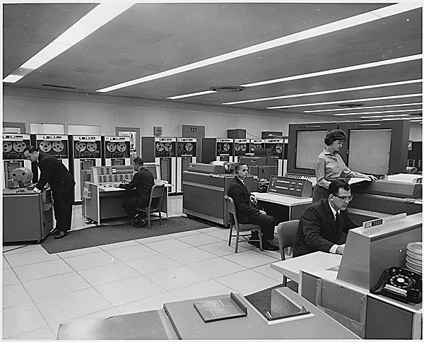
On February 20, 1962, John Glenn climbed into the Friendship 7 capsule atop an Atlas rocket at Cape Canaveral. Four hours later he had orbited the Earth three times – the first American to do so. The computing load for the mission was carried by two IBM 7090s at the Goddard Space Flight Center in Greenbelt, Maryland, backed up by an older IBM 709 in Bermuda. The 7090s computed the trajectory parameters, tracked Glenn’s real-time position, and predicted where the capsule would go next. Data flowed in at 1000 bits per second – a torrential rate for 1962 – and the machines kept up.
Katherine Johnson, whose story was told in Hidden Figures (2016), famously hand-checked the 7090’s orbital calculations before Glenn would agree to fly. “Get the girl to check the numbers,” Glenn allegedly said, referring to Johnson, the Black mathematician at NASA Langley whose manual trajectory calculations had proven flawlessly reliable.3 The film placed a 7090 front and center at NASA Langley. The machine had become a movie star – and, more importantly, a symbol of the moment when human computers and electronic computers worked side by side.
After Mercury came Gemini, and three IBM 7094s replaced the 7090s at Goddard. The Jet Propulsion Laboratory had three more 7094s in the Space Flight Operations Facility, plus two 7094/7044 direct-coupled systems. One 7094 was retained even during the Apollo program to run flight planning software that had never been ported to the newer System/360. The machine was too important to retire.
Meanwhile, 30 miles south of Goddard, in Suitland, the same type of machine was computing tomorrow’s weather.
Two IBM 7090s. Two ways of predicting the sky. One tracked a man’s orbit around the Earth. The other predicted what the atmosphere would do next. Both were running on 50 000 germanium transistors and 32 768 words of magnetic core memory. The hardware did not care whether the problem was celestial mechanics or fluid dynamics.
And that was not all. At Briarcliff Manor, New York, a pair of 7090s ran the SABRE airline reservation system for American Airlines – one of the first large-scale real-time transaction processing systems in history. At Thule Air Base in Greenland, 7090s scanned the Arctic sky for incoming Soviet missiles as part of the Ballistic Missile Early Warning System (BMEWS). Those BMEWS machines would run for roughly 30 years – one of the longest operational lifespans of any mainframe installation ever.
The 7090 appeared in Stanley Kubrick’s Dr. Strangelove (1964) – its blinking lights and the distinctive IBM 1403 printer visible in the background, the aesthetic of cold calculation as backdrop to nuclear paranoia. It appeared in Hidden Figures (2016), where it became a symbol of both institutional power and the human brilliance that checked its work. It even showed up in Event Horizon (1997), with 7094 specifications visible on screen. The same box of transistors forecast weather, tracked astronauts, booked airplane seats, watched for nuclear war, and played a role in some of the most celebrated films about technology ever made.
IBM built roughly 300 machines across the 7090/7094 production run. They cost about $2 900 000 to purchase (roughly $23 million in 2025 dollars). Monthly rental ran to $63 500. They were not cheap. They were everywhere that mattered.
The Computer That Sang
In 1961, at Bell Labs in Murray Hill, New Jersey, an IBM 7094 did something no computer had ever done before. It sang.
Physicist John L. Kelly Jr. and programmer Carol Lockbaum had built a vocoder synthesis program that could produce recognizable speech. Computer music pioneer Max Mathews wrote the musical accompaniment. The song they chose was “Daisy Bell” – the 1892 music-hall tune better known as “Bicycle Built for Two.” The recording is eerie, mechanical, unmistakably inhuman, and unmistakably singing. It is the earliest known recording of a computer-generated singing voice.
Science fiction writer Arthur C. Clarke happened to visit Bell Labs around this time, invited by his friend John R. Pierce, who was a Bell Labs engineer and science fiction author in his own right. Clarke heard the 7094 sing “Daisy Bell.” He never forgot it.
Seven years later, when Clarke and Kubrick were writing the screenplay for 2001: A Space Odyssey, they needed a way to show HAL 9000 dying. As astronaut Dave Bowman pulls the computer’s memory modules one by one, HAL’s voice slows, slurs, and regresses – and the last coherent thing the most famous fictional computer ever created does is sing “Daisy Bell.” It is one of the most haunting scenes in cinema history. Clarke put it in because he had heard an IBM 7094 do it at Bell Labs.
The 7094 that sang at Bell Labs was not unusual. It was a standard production machine, bought for scientific computation. The fact that it could also synthesize a human voice was a byproduct of the same raw computational power that made it useful for weather modeling, orbital mechanics, and airline reservations. The IBM 7090/7094 family was not designed to do any one thing. It was designed to compute. What you computed was up to you.
The same machine family that forecast the weather was the voice of science fiction’s most famous artificial intelligence. The 7090 and 7094 were everywhere in the early 1960s – tracking orbits, booking flights, singing songs, predicting rain. At MIT, the 7094 ran the Compatible Time-Sharing System (CTSS) – the first general-purpose time-sharing operating system, which proved that a single large computer could serve multiple interactive users simultaneously. At UCLA, a 7090 was used by Michael Minovitch to solve the gravitational three-body problem, laying the mathematical foundation for the Planetary Grand Tour that would send Voyager 1 and Voyager 2 past Jupiter, Saturn, Uranus, and Neptune. The machine was everywhere. It did everything.
TIROS: Seeing the Atmosphere
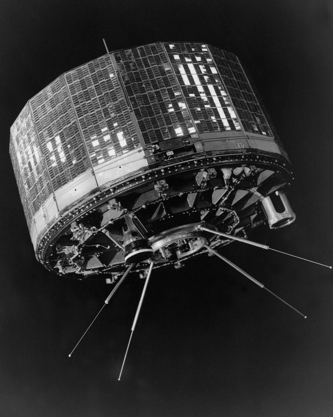
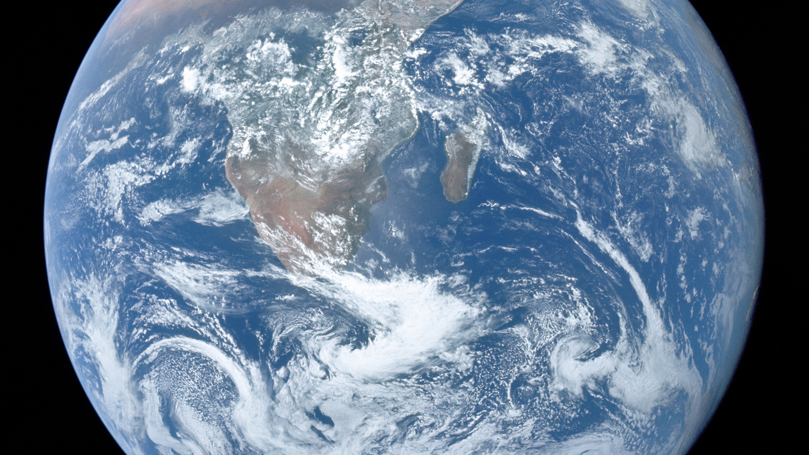
On April 1, 1960 – one day that was emphatically not a joke – a Thor-Able II rocket launched from Cape Canaveral at 11:40 UTC, carrying a 122-kilogram satellite called TIROS-1 (Television Infrared Observation Satellite). It was small – about the size of a washing machine drum, 42 inches in diameter, 22 inches high. It carried two small vidicon television cameras, one wide-angle and one narrow-angle, pointed at the Earth from an altitude of roughly 700 kilometers. It orbited the planet every 99 minutes.
For the first time in history, human beings could see the atmosphere from above.
In its 78 days of operation, TIROS-1 returned approximately 23 000 photographs, of which about 19 000 were usable for weather analysis. The images showed large-scale cloud patterns in their totality – vortex structures of mid-latitude cyclones, the spiral bands of tropical storms, the sharp edges of frontal systems. Meteorologists could suddenly see features they had only inferred from scattered surface observations and a handful of radiosonde soundings.
For NWP, the impact was transformative but not immediate. The early TIROS images were photographs, not gridded data. You could look at them and see a hurricane, but you could not easily feed them into a numerical model. The pipeline from satellite image to model input – what we now call satellite data assimilation – would take years to develop. But the direction was unmistakable. The atmosphere had been opaque. Now it was visible.
The significance for NWP was above all about data over the oceans. The Northern Hemisphere had a reasonable network of surface stations and radiosonde launch sites over land. But the oceans – which cover most of the planet and which generate most of the weather that hits coastlines – were a vast data void. A few ships, a few island stations, and nothing else. Satellites could see the whole globe every day. Even crude cloud-cover images told you where the storms were, and that was information the models desperately needed.
TIROS-1 was the first of a series. By the mid-1960s, an operational weather satellite system was in place, and by the 1970s, satellite data was becoming a critical input to global NWP models. Today, satellite observations account for the single largest source of data ingested by operational NWP systems worldwide. The data revolution that numerical weather prediction needed had begun on April 1, 1960, from a rocket that cost less than a single IBM 7090.
Man vs. Machine
As NWP improved through the early 1960s, a tension emerged that would persist for decades. Some meteorologists saw the computer as a threat. Others embraced it. Most were somewhere in between.
The British meteorologist Reginald Sutcliffe, who directed NWP research at the UK Met Office, had already articulated the anxiety in 1956:
“We are taught to look for the day when machines will calculate the future weather with a monotonous degree of success, but if that day comes one satisfying profession will be lost to man and we must look elsewhere.”4
Sutcliffe declared himself a forecaster first: “I am happy to claim membership in the forecasters group, once a forecaster always a forecaster.”4
The nuanced truth, as it emerged by the mid-1960s, was more interesting than either the enthusiasts or the skeptics had predicted. NWP beat humans at the 500 mb level – the large-scale flow of the upper atmosphere at roughly 5500 meters altitude, on time scales of 24 to 72 hours. At this scale, the equations of motion dominate, the flow is approximately geostrophic (balanced between pressure gradient and Coriolis force), and a decent model with decent initial conditions will outperform any human’s ability to extrapolate from pattern recognition.
But humans remained essential for everything else. Surface weather – the rain, snow, fog, and wind that people actually experience – depended on topography, land-sea contrasts, and boundary-layer physics that the coarse models of the 1960s could not resolve. Mesoscale phenomena – thunderstorms, squall lines, lake-effect snow – happened at scales far below the grid spacing. Nowcasting – the next few hours – was still the domain of the experienced forecaster watching radar and looking out the window. And perhaps most critically, human forecasters brought something the computer could not: the ability to know when the model was wrong.
Every experienced forecaster developed an intuition for the model’s failure modes. When the 500 mb pattern was split-flow, the barotropic model handled it badly. When a strong jet streak was present, the quasi-geostrophic approximation broke down. When the model’s initial analysis was contaminated by a bad radiosonde report, the entire forecast could go haywire. A skilled forecaster could recognize these situations and adjust. The computer could not.
The forecasters who thrived in the NWP era were not the ones who fought the computer or the ones who slavishly followed it. They were the ones who learned to read the model – to use its output as one input among many, to combine it with their own knowledge of local conditions and their hard-won sense of when the atmosphere was doing something the model could not capture.
The Weather Bureau’s own data confirmed this. The interpretation of model output by human forecasters added a consistent, measurable improvement over raw model guidance. Man and machine were better together than either was alone. This finding has held true through every subsequent generation of NWP, right up to the present day.
There was also the problem of public communication. A computer produces a gridded field of numbers. The public wants to know: will it rain at my daughter’s wedding? Will the highway be icy tomorrow morning? Should I evacuate? Translating the model’s output into actionable human language – with appropriate confidence and caveats – required a human forecaster who understood both the model and the audience. No computer in the 1960s could do that. No computer today does it perfectly. The forecaster’s role did not disappear with NWP. It evolved.
Shuman’s Primitive Equations
All through the late 1950s and early 1960s, Fred Shuman – the JNWPU’s first employee, the man who had been at the IBM 701 console in 1955 – had been working toward a goal. He wanted to solve the full primitive equations of atmospheric motion.
Every operational model until then had used the quasi-geostrophic approximation – a simplification that filters out certain fast-moving wave solutions (gravity waves, sound waves) from the equations. The quasi-geostrophic system is cheaper to solve and numerically more stable. But it is an approximation. It misses phenomena that the full equations capture: ageostrophic circulations, strong jet-level divergence, the vertical motions that drive precipitation. To get the forecast truly right, you needed the primitive equations – the hydrostatic equations of motion, the thermodynamic energy equation, the continuity equation, and the equation of state, solved together without the geostrophic filter.
The problem was computational. The primitive equations are stiffer, harder to integrate, and more sensitive to initial conditions and numerical methods. They demanded more computer power than anyone had in the late 1950s.
Then Seymour Cray built his masterpiece.
Cray was a quiet, meticulous engineer from Chippewa Falls, Wisconsin – a small town on the Chippewa River, population about 12 000, the kind of place where a man could think without interruption. He had joined Control Data Corporation in 1957 and quickly established himself as the company’s most important designer. He preferred to work alone or with a small team. He avoided meetings. He built canoes and dug tunnels under his house for relaxation. He was, by every account, the most talented computer architect of his generation.
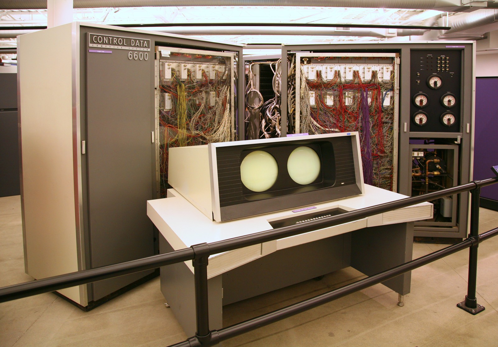
The CDC 6600, first delivered in 1964, was his masterpiece – and it was the fastest computer in the world. It executed roughly 3 000 000 instructions per second – nearly ten times faster than anything else available. It used approximately 400 000 transistors, silicon rather than germanium, cooled by Freon refrigerant. The clock cycle was 100 nanoseconds – 10 megahertz. Its architecture was revolutionary: a single fast central processor supported by ten smaller 12-bit peripheral processors that handled all I/O, freeing the main CPU to do nothing but compute. Cray had, in effect, invented the modern concept of offloading I/O to dedicated hardware. The central processor had multiple functional units that could operate in parallel – a precursor to the pipelining that would define all subsequent supercomputer design.
The CDC 6600 was so fast that when IBM learned of it, Thomas Watson Jr. reportedly fired off an angry memo lamenting that IBM had lost “our industry leadership position” to a lab of “34 people, including the janitor.”5 The janitor line may be apocryphal. The fury was real. IBM responded by announcing the System/360 Model 91, explicitly aimed at recapturing the scientific computing market. It was too late. Cray had already won.
NMC got its CDC 6600, and Fred Shuman finally had the machine he needed. Shuman had been thinking about this problem for over a decade. He had worked at the Institute for Advanced Study in Princeton from 1952 to 1954, attending lectures by J. Robert Oppenheimer and running test models on one of the IAS-class machines. He had been the JNWPU’s first employee in 1954. He had diagnosed the failures of the three-level quasi-geostrophic model on the IBM 701. He had built the improved barotropic model that finally showed skill in 1958. He had developed the Shuman smoother – the finite-difference filtering technique that removed spurious short-wave noise without distorting the meteorologically significant scales. Every step had been building toward this: solving the real equations on a machine fast enough to handle them.
In mid-1966, the six-layer primitive equation model went operational. Shuman and his colleague John Hovermale published the definitive description in 1968: “An Operational Six-Layer Primitive Equation Model” in the Journal of Applied Meteorology. The model integrated the full hydrostatic primitive equations over six vertical levels, covering the Northern Hemisphere. No more quasi-geostrophic approximation. No more filtering out the physics that mattered.
The results, in Shuman and Hovermale’s own words, produced “highly significant improvements” in NMC’s forecast products in its first fourteen months of operational use.6 The six-layer PE model was the first operational model anywhere in the world to use the full primitive equations. West Germany began running a primitive-equation model the same year, but NMC’s was the benchmark. And by June 1966, NMC had also achieved its first global forecast run – no longer just the Northern Hemisphere, but the entire planet.
The CDC 6600 could produce a numerical forecast for all of North America out to 48 hours in less than 30 seconds. It was, by one estimate, roughly 50 000 times more powerful than the IBM 701 that had struggled through those first disappointing forecasts just eleven years earlier. Cray’s machine ran at NMC until it was replaced by the even faster CDC 7600 – Cray’s second masterpiece, five to ten times faster still, which held the title of world’s fastest computer from 1969 to 1975.
Nineteen Years
By 1969, numerical weather prediction was consistently useful.
The S1 score – a measure of forecast skill where 70 is worthless and 20 is near-perfect – had been dropping steadily since the late 1950s. The 72-hour 500 mb forecast, which had been no better than guesswork in 1955, was now reliably beating human forecasters. The 24-hour surface forecast, the product that ordinary people actually cared about, was improving year by year as models gained vertical resolution and as satellite data began filling the vast observational gaps over the oceans.
George Cressman had left the NMC directorship in 1964 to become head of the Weather Bureau (later the National Weather Service under NOAA, which was created in 1970). Fred Shuman succeeded him as NMC director, a post he would hold until 1981 – seventeen years, through the CDC 6600, the CDC 7600, and the first Cray machines. He continued research at NMC until 1986, five years after his retirement as director. For his work he received the Department of Commerce Silver Medal in 1957 and the Gold Medal in 1967.
Between them, Cressman and Shuman had led American operational NWP from the IBM 701 to the supercomputer era. Cressman’s objective analysis method of 1959 – a successive-correction technique for interpolating scattered observations onto a regular grid, based on ideas from the Swedes Bergthorsson and Doos – was still the foundation of data assimilation. Shuman’s primitive equation model of 1966 was the template for every global model that followed.
The revolution that had begun on the ENIAC in 1950 had taken nineteen years to deliver on its promise. Five generations of computers – ENIAC, IBM 701, IBM 704, IBM 7090/7094, CDC 6600. Two satellite systems. A data assimilation method. A filtering theory. A primitive equation model. And the stubbornness of people like Cressman and Shuman, who kept running the model every single day even when the forecasts were bad, because the only way to find the problems was to face them operationally.
By 1969, the forecast was good. Not perfect. Not even close. But good enough that no serious meteorologist doubted the computer’s role. Good enough that the question was no longer “should we use NWP?” but “how do we make it better?”
Consider the arc.
In 1950, Charney and his team had run the first weather forecast on the ENIAC at Aberdeen. The calculation took 24 hours to produce a 24-hour forecast – it was slower than the weather itself.
In 1955, the IBM 701 at JNWPU produced forecasts that were “very disappointing and not usable by forecasters.”1
In 1958, the barotropic model on the IBM 704 finally showed skill.
In 1960, the IBM 7090 made the models fast enough to be operationally useful. TIROS-1 opened a window onto the global atmosphere.
In 1962, the 7094 ran the first operational baroclinic model.
In 1966, the CDC 6600 ran the first primitive-equation model.
By 1969, the 72-hour 500 mb forecast was reliably beating human forecasters, and the pipeline from observation to forecast to public dissemination was working every day, twice a day, without fail.
Five generations of computers. Nineteen years. A data revolution from satellites. And the stubbornness of people who kept running the model every single day even when the forecasts were bad, because the only way to find the problems was to face them operationally.
The next step would be Seymour Cray’s purpose-built supercomputers – machines that would push NWP from hemispheric to global, from six layers to dozens, from deterministic to ensemble. But that is a story for a future post.
The decade the forecast got good was the 1960s. And the people who made it happen – Cressman the institution-builder, Shuman the modeler, Cray the architect – never got the fame of the astronauts whose orbits their machines also tracked.
Fred Shuman died on July 29, 2005, aged 86, of congestive heart failure, at his home in Fort Washington, Maryland. The Washington Post ran an obituary headlined “Meteorological ‘Pioneer’ Frederick G. Shuman Dies.” George Cressman died on April 17, 2008, aged 88, of Alzheimer’s disease, in Rockville, Maryland. He had won the International Meteorological Organization Prize in 1977 and served as president of the American Meteorological Society in 1978. Seymour Cray died in a car accident in Colorado Springs on October 5, 1996, aged 71. None of them became household names.
The weather forecast is invisible infrastructure. When it works, nobody notices. When it fails, everyone complains. The men who built it worked in a beige government office building in Suitland, Maryland, and their reward was the quiet satisfaction of watching the S1 scores drop, year after year, as the models got better and the forecasts got good.
Footnotes
References
The IBM 7090/7094:
- IBM 7090. Wikipedia. Wikipedia
- IBM 709. Wikipedia. Wikipedia
- The IBM 7090. Columbia University Computing History. Columbia
- IBM 700/7000 series. Wikipedia. Wikipedia
Project Mercury and NASA Computing:
- Project Mercury. IBM Corporate History. IBM
- Katherine Johnson, Hidden Figures, and John Glenn’s Flight. National Air and Space Museum. NASM
TIROS-1:
- TIROS-1. Wikipedia. Wikipedia
- Celebrating 65 Years of the World’s First Weather Satellite. NESDIS/NOAA. NOAA
- TIROS, the Nation’s First Weather Satellite. NASA. NASA
“Daisy Bell” and HAL 9000:
- Daisy Bell. Wikipedia. Wikipedia
- The IBM 7094 is The First Computer to Sing. History of Information. HistoryofInformation
CDC 6600:
- CDC 6600. Wikipedia. Wikipedia
- CDC 6600’s Five Year Reign. Computer History Museum. CHM
- CDC 6600. NCAR/CISL Supercomputing History. UCAR
Shuman’s Primitive Equation Model:
- Shuman, F.G. and Hovermale, J.B. (1968). An Operational Six-Layer Primitive Equation Model. Journal of Applied Meteorology, 7(4), 525-547. AMS
- Shuman, F.G. (1989). History of Numerical Weather Prediction at the National Meteorological Center. Weather and Forecasting, 4(3), 286-296. AMS
NMC/NCEP History:
- Environmental Modeling Center (EMC) History. NCEP. EMC
- Summary of WPC History and Leadership. NCEP/WPC. WPC
- Harper, K., Uccellini, L.W., Kalnay, E., Carey, K. & Morone, L. (2007). 50th Anniversary of Operational Numerical Weather Prediction. Bulletin of the American Meteorological Society, 88(5), 639-650. AMS
Cressman and NWP:
- Cressman, G.P. (1959). An Operational Objective Analysis System. Monthly Weather Review, 87(10), 367-374.
- Numerical Weather Prediction. NWS Heritage, VLab. VLab
- The History of Numerical Weather Prediction. NOAA Mariners Weather Log, December 2007. NOAA
NWP History and Man vs. Machine:
- Yang, C. (2025). The First Compute Arms Race: The Early History of Numerical Weather Prediction. arXiv
- History of numerical weather prediction. Wikipedia. Wikipedia
SABRE and BMEWS:
- IBM 7090 Wikipedia entry, sections on SABRE and BMEWS.
Image Credits:
- IBM 7090 at NASA. NASA/Wikimedia Commons. Wikimedia
- TIROS-1 satellite. NASA. Wikimedia
- CDC 6600. Computer History Museum/Wikimedia Commons. Wikimedia
Previously in this series: The Man Who Forecasted Weather with a Pencil – The Number That Connects Turbulence to War – The Line That Models Cannot Draw (Part 1) – Reading the Sky – The Ghost in the Grid – The Man Who Tamed the Equations – The First Climate Model Had 5 KB of RAM – The Butterfly That Broke the Forecast – From Cables to Chaos – The Swedes Got There First – The Magician Who Told No Secrets – The Blueprint Von Neumann Gave Away – The Machine That Learned Too Early – The Machine That Built IBM – Three Mathematicians from Poznan – The Forecast That Reached the Nobel
-
Environmental Modeling Center (EMC) History. NCEP. EMC. ↩ ↩2
-
Shuman, F. G. “History of Numerical Weather Prediction at the National Meteorological Center.” Weather and Forecasting, 4(3), 1989, 286-296. AMS. ↩
-
Shetterly, M. L. Hidden Figures: The American Dream and the Untold Story of the Black Women Mathematicians Who Helped Win the Space Race, William Morrow/HarperCollins, 2016. See also “Katherine Johnson, Hidden Figures, and John Glenn’s Flight,” National Air and Space Museum. NASM. ↩
-
Sutcliffe, R. C. Presidential Address, Royal Meteorological Society, 1956. Quarterly Journal of the Royal Meteorological Society, 82 (1956). ↩ ↩2
-
Watson, T. J., Jr., internal IBM memo, 1963, as recounted in CDC 6600 corporate and Computer History Museum histories. CHM. ↩
-
Shuman, F. G. and Hovermale, J. B. “An Operational Six-Layer Primitive Equation Model.” Journal of Applied Meteorology, 7(4), 1968, 525-547. AMS. ↩