Yesterday, I told you about Jule Charney - the man who figured out which equations to keep and which to throw away, and then proved that a computer could forecast the weather. That was 1950. A 24-hour forecast, a barotropic model, the ENIAC.
But Charney’s team predicted one day of weather from today’s observations. That’s the initial-value problem: given what the atmosphere looks like right now, what happens tomorrow?
There is a much harder question.
What if you don’t know what the atmosphere looks like right now? What if you start with nothing - no winds, no temperature gradients, no storms - just a featureless ball of air, heated unevenly by the sun? Will the right weather emerge on its own?
One of Charney’s own team members decided to find out. His name was Norman Phillips. And what he did in 1955, on a machine with 5 kilobytes of RAM, changed the trajectory of climate science forever.
A Kid from Chicago Who Went to War
Norman A. Phillips was born on July 9, 1923, in Chicago, Illinois. He enrolled at the University of Chicago in 1940, originally studying chemistry - because apparently you have to start somewhere wrong before you find the right path.
Then the war came.
Phillips enlisted in the U.S. Army Air Corps in March 1942. After training at the University of Michigan and Chanute Field in Illinois, he was commissioned as a Second Lieutenant on June 5, 1944 - the day before D-Day. He was deployed to the Azores, where he created daily weather forecasts for Allied trans-Atlantic flights. Not a desk job. Not a training exercise. Real forecasts for real pilots flying real missions across an ocean where getting the weather wrong meant people didn’t come home.
He was discharged as a First Lieutenant in August 1946, went back to Chicago, and tore through a B.S. (1947), an M.S. (1948, under Erik Palmen), and a Ph.D. (1951, under George Platzman, a mathematical meteorologist who later wrote the definitive history of the ENIAC forecasts) in meteorology. His dissertation? A two-layer baroclinic model - the exact kind of mathematical framework that would, four years later, become the skeleton of the first climate simulation.
Chicago in the late 1940s was the place to be if you cared about atmospheric dynamics. Carl-Gustaf Rossby was there. Platzman was there. The intellectual ferment was extraordinary. And in 1948, a paper arrived that grabbed Phillips by the collar: Jule Charney’s “On the scale of atmospheric motions.” Phillips later said it was this paper that awakened his interest in dynamic meteorology.
In October 1951, Phillips joined Charney’s team at the Institute for Advanced Study in Princeton. He was about to meet the machine.
5 KB of RAM and No DO-Loops
The computer at the IAS was built under the direction of John von Neumann between 1946 and 1951. It was publicly displayed for the first time on June 10, 1952. Sometimes called the “IAS machine” or the “von Neumann machine,” it was one of the first stored-program computers ever built.
Here are the specs. Try not to laugh.
- Internal memory: 1,024 words of 40 binary digits each - approximately 5 kilobytes of RAM
- Drum memory: 2,048 words - approximately 10 kilobytes (later upgraded to 16,384 words)
- Add time: 42 microseconds
- Multiply time: 700 microseconds
- Speed: roughly 24,000 additions per second
- Construction: 3,430 vacuum tubes, 2,091 transistors, 915 diodes
- Power consumption: 61 kilowatts
For context: the phone in your pocket has millions of times more memory. A cheap USB stick from a gas station has more storage. A modern smartwatch could run circles around this thing. Your Wi-Fi router probably has more computing power.
And the programming experience? Let Phillips tell you himself:
“Code was written in what would now be called ‘machine language’ except that it was one step lower – the 40 bits of an instruction word (two instructions) were written by us in a 16-character (hexadecimal) alphabet 0, 1, …, 9, A, B, C, D, E, F instead of writing a series of 0’s and 1’s.”1
No high-level language. No compiler. No debugger. Raw hexadecimal, hand-coded, one instruction at a time.
“There was no automatic indexing – what we now call a ‘DO-LOOP’ was programmed explicitly with actual counting. Subroutines were used, but calls to them had to be programmed using explicitly stored return addresses.”1
If you’ve ever been frustrated by a Python script that won’t import a library, imagine hand-coding every loop counter in hex on a machine that stores its memory in cathode-ray tubes. That’s the level of suffering we’re talking about. This is like playing a souls-like game where the controller is also on fire.
The Experiment: Starting from Nothing
Phillips returned to Princeton in April 1954 with a plan. He had just published a theoretical paper on energy transformations in baroclinic waves - the intellectual foundation for what came next - and he convinced Charney it was worth trying.
The idea was audacious. Instead of starting with observed weather and forecasting forward (like Charney’s 1950 ENIAC run), Phillips would start with an atmosphere at rest and see if realistic weather would emerge on its own from nothing but differential heating.
The model was almost absurdly simple. John Lewis, writing the definitive retrospective in 1998, described it as exhibiting:
“an almost irreverent disregard for the complexities of the real atmosphere.”2
Here’s what Phillips built:
- Two levels in the vertical (250 mb and 750 mb - upper and lower atmosphere)
- 17 x 16 grid points in the horizontal
- Grid spacing: 625 km north-south, 375 km east-west
- A rectangular channel representing the distance from equator to pole (10,000 km) and one wavelength east-west (6,000 km)
- Roughly 500 variables to describe the entire state of the atmosphere
- Heating: a simple linear function of latitude (warm in the south, cold in the north)
- Friction: proportional to wind speed at the surface
- No mountains. No oceans. No water vapor. No clouds. No precipitation. A totally dry model.
The state of the entire simulated atmosphere - everything - fit into roughly half of the IAS machine’s 1,024-word memory. The other half held the program code.
500 numbers. That’s it. The instantaneous state of Phillips’ atmosphere was captured in 500 numbers. For comparison, a modern climate model uses tens of millions of variables. The ECMWF’s operational model runs on grids with billions of points. Phillips had 500.
The experiment ran in two phases. First, a spin-up: 130 simulated days with no east-west variation, just letting the heating build up a temperature gradient. By the end of that phase, the atmosphere had a broad westerly jet at the upper level and weak easterlies at the surface - a reasonable starting point.
Then Phillips added a small random perturbation - generated by “repeated squaring of an initially given generating number,” which is the 1955 version of Math.random() - and let the full model run.
Time step: 2 hours or less.
Duration: 31 simulated days.
Total computer time for those 31 days: 11 to 12 hours on the IAS machine.
What Came Out
This is where it gets extraordinary.
From an atmosphere that started at rest - no winds, no storms, no structure - the model produced:
A jet stream. Transport of momentum by the developing eddies created a jet of 40-60 m/s at the upper level during days 10-25. That’s realistic. That’s what the real atmosphere does.
The correct surface wind pattern. Easterlies at subtropical latitudes, westerlies in the midlatitudes, easterlies again near the “pole.” The classic three-belt pattern that every introductory meteorology textbook shows. It emerged spontaneously from 500 numbers and simple heating.
A realistic cyclone. A baroclinic wave developed with a wavelength of about 6,000 km, moving eastward at 21 m/s (1,800 km per day). The flow tilted westward with height - exactly as real extratropical cyclones do. It started as a warm low and gradually evolved to look, in Phillips’ words, “very much like those of an occluded cyclone.”3
A three-cell meridional circulation. Two direct cells (Hadley-type) near the equatorial and polar boundaries, and one indirect cell (Ferrel cell) in the middle latitudes. The real atmosphere has exactly this structure. Phillips’ 500 numbers found it.
And then - the result that made Rossby’s jaw drop.
Fronts.
Phillips wrote:
“Definite indications of something similar to cold and warm fronts are to be seen in the 1,000-mb contours, with the main temperature gradient occurring on the cold side of the ‘frontal troughs’.”3
On some days, the fronts were “so pronounced as almost to force a kinking of the contour lines.”3
If you’ve been following this series - from the Bergen School inventing the concept of fronts, to human forecasters learning to read them from satellites, to the models struggling to reproduce them - you know why this matters. Fronts are emergent phenomena. No equation in Phillips’ model contained the word “front.” There was no frontal parameterization. There was no frontal boundary condition. There were just the quasi-geostrophic equations, differential heating, and friction.
And fronts appeared anyway. Out of 500 numbers. On 5 KB of RAM.
Phillips, characteristically modest, summed up:
“Considering the simplicity of the model, these modest successes are quite gratifying.”3
Modest successes. The man simulated the general circulation of the atmosphere from scratch and called it “modest successes.” I can’t even get a Docker container to start on the first try.
The Blow-Up
It wasn’t all triumph.
After about 25-26 days of simulated time, the model began to fall apart. The field of mean zonal wind developed oscillations at the smallest resolvable scale - a 2-delta-x wave, which is the numerical equivalent of the model screaming for help. By day 26, the meridional circulation had become “very irregular owing to large truncation errors.” By day 28, energy was increasing fictitiously and uncontrollably.
Phillips wrote in his abstract:
“Truncation errors eventually put an end to the forecast by producing a large fictitious increase in energy.”3
He tried adding lateral diffusion to smooth things out. It helped a little, but not enough. The model was dying, and he didn’t fully understand why.
It took him three more years to figure it out.
In 1959, Phillips published a short but devastating paper: “An example of non-linear computational instability.” The problem was aliasing. When two waves interact through the nonlinear advection terms (the parts of the equations where the wind carries itself - velocity times velocity, which means the output depends on the square of the input rather than the input alone), they produce new waves at the sum and difference of their wavenumbers. On a discrete grid, waves shorter than twice the grid spacing cannot be represented. Those phantom short waves get folded back - “aliased” - into longer waves, contaminating the solution with fictitious energy.
Phillips’ solution: transform the data into Fourier space, chop off the upper half of the spectrum, and transform back. With that filter in place, the model could run indefinitely.
This was the first identification and solution of the aliasing problem in computational fluid dynamics. Every spectral model running today - every climate simulation that uses spherical harmonics, every weather model with spectral filtering - traces its intellectual lineage back to Phillips realizing why his model blew up after 25 days on a machine with 5 KB of RAM.
“Yes, Norman, and It Should Be That!”
The reactions from the meteorological community tell you everything you need to know about what Phillips had achieved.
Carl-Gustaf Rossby, one of the most influential meteorologists of the twentieth century, had a conversation with Phillips in Stockholm in early 1956 (reconstructed by Wiin-Nielsen):
R: “Norman, do you really think there are fronts there?”4
P: “Yes, look at the temperature fields packed up very nicely.”4
R: “But Norman, what’s the process that creates these fronts? Where do they come from?”4
P: “Well, they come out of a very simple dynamics.”4
R: “And what is that?”4
P: “I have very simple linear heating between the equator and pole, simple dissipation, but of course there is no water vapor or no precipitation, no clouds, totally dry model.”4
R: “Yes, Norman, and it should be that! Because here we are getting this front – and it has nothing to do with clouds/rising motion, it is a sheer dynamic effect that comes as a result of the development.”4
Think about what Rossby grasped in that moment. Fronts - those sharp boundaries where air masses collide, the lines that forecasters draw on weather maps, the features that the Bergen School had spent decades studying - were not caused by moisture or clouds or precipitation. They were a pure dynamical consequence of differential heating and baroclinic instability. Phillips’ dry, cloudless, mountainless, featureless model proved it.
Eric Eady said at the Napier Shaw lecture in 1956:
“I think Dr. Phillips has presented a really brilliant paper which deserves detailed study from many different aspects.”5
Eady added something profound about the experimental design:
“An experiment which merely attempted to ape the real atmosphere would have been very poorly designed and very much less informative.”5
In other words: the simplicity was the point. By stripping away everything except the essential dynamics, Phillips revealed what the atmosphere does when nothing else gets in the way.
Joseph Smagorinsky - readers who follow this series already know him from the ENIAC team - who would go on to found GFDL:
“A new era had been opened.”6
And von Neumann himself recognized the significance immediately. When Phillips showed him the results in 1955, von Neumann moved on two fronts simultaneously. He organized a conference at Princeton in October 1955 - “The Application of Numerical Integration Techniques to the Problem of General Circulation.” And he drafted a proposal, dated August 1, 1955, to the Weather Bureau, Air Force, and Navy for a new joint project dedicated to simulating the general circulation.
That proposal was accepted the following month. Smagorinsky was asked to lead the new General Circulation Research Section, and reported for duty on October 23, 1955.
From 500 Numbers to a Nobel Prize
The lineage from Phillips’ experiment to modern climate science is direct and unbroken.
Phillips’ results convinced von Neumann to create the General Circulation Research Section. Smagorinsky built it up, first in collaboration with von Neumann and Charney, then independently. In 1963, Smagorinsky published the next major step - a GCM using the full primitive equations instead of Phillips’ quasi-geostrophic approximation. In 1965, the research unit was formally established as the Geophysical Fluid Dynamics Laboratory (GFDL) in Princeton.
At GFDL, a young Japanese scientist named Syukuro Manabe was building on the foundation Phillips had laid. In 1967, Manabe and Wetherald published the seminal paper on CO2 and climate sensitivity. In 1969, Manabe and Bryan coupled an atmospheric GCM to an ocean model - the first coupled climate model.
Within a decade of Phillips’ 1956 paper, major GCM efforts had sprung up at NCAR in Boulder, Lawrence Livermore Laboratory, UCLA (where Akio Arakawa, who explicitly credited Phillips as his inspiration, built his own models), and the UK Met Office. Every single one traced back, directly or indirectly, to what Phillips had shown was possible.
And in 2021, Syukuro Manabe received the Nobel Prize in Physics “for the physical modelling of Earth’s climate, quantifying variability and reliably predicting global warming.”
The line runs straight: Phillips’ 500 numbers on 5 KB of RAM -> von Neumann’s proposal -> Smagorinsky’s research section -> GFDL -> Manabe -> the Nobel Prize. Sixty-five years from a dry, cloudless, two-layer model on a machine with vacuum tubes to the highest honor in science.
As Steve Easterbrook wrote in his 2019 memorial for Phillips:
“The best means we have of anticipating changes is through Earth System Models; the direct descendants of the simple two-layer model used with such effect by Norman Phillips in 1956.”7
What Comes Next
Phillips proved something that nobody had proved before: the atmosphere could be simulated from first principles. You didn’t need to observe the weather to reproduce it. You just needed the right physics, enough patience, and a machine that could count to 500 without catching fire.
But there was a catch nobody saw coming. Phillips’ model blew up after 25 days, and while he eventually figured out why, the fix revealed a deeper problem - one that would haunt every climate model built after his. The atmosphere is chaotic. Small errors grow. And the very nonlinearity that makes the weather interesting is the same nonlinearity that makes it impossible to predict beyond a certain horizon.
That’s a story for next time.
Footnotes
References
- Phillips, N. A. (1956). The general circulation of the atmosphere: a numerical experiment. Q. J. R. Meteorol. Soc., 82(352), 123-164. PDF / Wiley
- Phillips, N. A. (1959). An example of non-linear computational instability. In The Atmosphere and the Sea in Motion (Rossby Memorial Volume), B. Bolin, Ed., Rockefeller Press, 501-504.
- Lewis, J. M. (1998). Clarifying the Dynamics of the General Circulation: Phillips’s 1956 Experiment. Bull. Amer. Meteor. Soc., 79(1), 39-60. PDF
- Wiin-Nielsen, A. (1997). The birth of numerical weather prediction. Tellus A, 49(5), 36-48.
- Phillips, N. A. (1990). Dispersion Processes in Large-Scale Weather Prediction. Sixth IMO Lecture, WMO No. 700, World Meteorological Organization, Geneva.
- Eady, E. T. (1956). Discussion contribution to Phillips’ Napier Shaw Memorial Lecture. Q. J. R. Meteorol. Soc., 82(352), 535-539.
- Smagorinsky, J. (1983). The beginnings of numerical weather prediction and general circulation modeling. Advances in Geophysics, 25, 3-37. ScienceDirect
- Franklin Institute. Norman Phillips - 2003 Bower Award
- MIT News (2019). Norman Phillips, former meteorology department head, dies at 95. MIT
- Easterbrook, S. (2019). In memory of Norman Phillips. Blog
- Lynch, P. (2019). A Pioneer of Climate Modelling and Prediction. ThatsMaths
- Carbon Brief (2018). Timeline: The history of climate modelling. Carbon Brief
- IAS Electronic Computer Project. IAS
- Smithsonian National Museum of American History. IAS Computer. Smithsonian
Current status:
- My cluster: Has about a million times more RAM than the IAS machine. Produces roughly the same number of bugs.
- Phillips’ 500 variables: Now tens of millions. The fronts still emerge. The models still blow up sometimes.
- The Nobel Prize committee: Took 65 years to trace the line back. Better late than never.
Yours Truly
-
Phillips, N. A. (1990). Dispersion Processes in Large-Scale Weather Prediction. Sixth IMO Lecture, WMO No. 700, World Meteorological Organization, Geneva. Phillips’ retrospective on IAS-machine-era programming. ↩ ↩2
-
Lewis, J. M. (1998). Clarifying the Dynamics of the General Circulation: Phillips’s 1956 Experiment. Bull. Amer. Meteor. Soc., 79(1), 39-60. PDF. ↩
-
Phillips, N. A. (1956). The general circulation of the atmosphere: a numerical experiment. Q. J. R. Meteorol. Soc., 82(352), 123-164. PDF. ↩ ↩2 ↩3 ↩4 ↩5
-
Wiin-Nielsen, A. (1997). The birth of numerical weather prediction. Tellus A, 49(5), 36-48. Reconstruction of the 1956 Stockholm conversation between Rossby and Phillips. ↩ ↩2 ↩3 ↩4 ↩5 ↩6 ↩7
-
Eady, E. T. (1956). Discussion contribution to N. A. Phillips, “The general circulation of the atmosphere: a numerical experiment,” Napier Shaw Memorial Lecture. Q. J. R. Meteorol. Soc., 82(352), 535-539. ↩ ↩2
-
Smagorinsky, J. (1983). The beginnings of numerical weather prediction and general circulation modeling. Advances in Geophysics, 25, 3-37. ScienceDirect. ↩
-
Easterbrook, S. (2019). In memory of Norman Phillips. Blog. ↩