Part 1 told the Bergen School story. Part 2 showed how humans read fronts from observations and satellites. Now: why the models can’t do what the human does - and the machines trying to learn.
Why the Models Cannot Draw the Line
Every NWP model - ECMWF’s Integrated Forecasting System, NOAA’s GFS, the WRF model used for research - still has Bjerknes’ original seven equations at its core:
- 3 momentum equations (Newton’s second law applied to air - one each for the eastward, northward, and vertical wind components)
- 1 continuity equation (mass is neither created nor destroyed)
- 1 thermodynamic energy equation (heat changes temperature)
- 1 equation of state (the ideal gas law - linking pressure, density, and temperature)
- 1 moisture equation (water vapor is carried by the wind and can condense or evaporate)
Seven equations, seven unknowns: u, v, w, T, p, rho, q. That’s the Bjerknes core. Richardson tried to solve them by hand. The ENIAC team solved a simplified version. They are still there, unchanged, inside every model running today.
But a modern operational model is far more than seven equations. Over a century of atmospheric science has piled on top of Bjerknes’ foundation:
Water species: Bjerknes had one moisture variable - water vapor. A modern microphysics scheme in WRF tracks five or six species separately: vapor, cloud liquid water, cloud ice, rain, snow, and graupel. Each has its own prognostic equation describing how it is created, transported, and converted into other species. That’s 5-6 equations replacing Bjerknes’ single moisture equation.
Radiation: The atmosphere absorbs and emits radiation at every level - shortwave from the sun, longwave from the Earth and clouds. Bjerknes didn’t model this. Modern models solve radiative transfer equations through dozens of spectral bands, accounting for absorption by water vapor, CO2, ozone, and aerosols. ECMWF’s radiation scheme alone is one of the most expensive parts of the model.
Turbulence: The grid can’t resolve individual turbulent eddies (that would require meter-scale resolution). So models use turbulence closure schemes - additional equations that parameterize the effect of subgrid-scale mixing on momentum, heat, and moisture. The planetary boundary layer scheme in WRF adds its own set of equations to represent how the lowest 1-2 km of the atmosphere churns during the day and stabilizes at night.
Convection: At grid spacings larger than about 4 km, individual thunderstorms can’t be resolved. Models use cumulus parameterization schemes - statistical representations of what convection does to the column of air above a grid point. These schemes trigger, produce rainfall, redistribute heat vertically, and detrain moisture into the environment - all based on equations that Bjerknes never imagined.
Land surface: The ground matters. Soil moisture, vegetation, snow cover, urban heat islands - all affect the atmosphere from below. Modern models couple to land surface models with their own prognostic equations for soil temperature, soil moisture at multiple depths, snow depth, and canopy processes.
Chemistry and aerosols: ECMWF’s IFS carries ozone and aerosol tracers with their own transport and reaction equations. Some configurations run full atmospheric chemistry - hundreds of chemical species interacting.
So Bjerknes’ 7 equations have grown into dozens of coupled prognostic equations wrapped in parameterization schemes that would fill a textbook. But the core - the momentum, the mass, the energy, the gas law - is still Bjerknes 1904, still recognizable, still doing the heavy lifting.
And nowhere in any of those equations - old or new - does the word “front” appear.
The model computes temperature at grid point A and temperature at grid point B. If there’s a 15-degree difference between them across 100 km, the model doesn’t think “oh, that’s a front.” It just has two numbers. The sharp gradient is there in the data, but the model has no concept of what it means.
Fronts are emergent phenomena - they fall out of the physics the way turbulence falls out of the Navier-Stokes equations. The model predicts the conditions for fronts to exist without knowing what fronts are.
The Resolution Problem
And here’s the catch. A typical cold front is 50-100 km wide. A sharp one can be 10 km or less. To resolve a feature in a numerical model, you need at least several grid points across it.
- Richardson’s 200 km grid (1917): Couldn’t resolve a front. The feature was thinner than the grid.
- ENIAC’s 736 km grid (1950, 19x16 points): Hopeless. You could fit several fronts between grid points and the model would never know.
- ECMWF IFS at ~9 km (today): Fronts begin to emerge as recognizable features - tight gradients in theta-e, wind shifts, convergence zones. But they’re still smoothed compared to reality.
- WRF at 1-3 km: Resolves frontal structure much better. Recent research shows that convection-permitting models produce continuous cold fronts while parameterized-convection models show broken, fragmented fronts (Crespo et al., 2023).
The gap between what the model produces and what a forecaster draws on a chart is still real. It’s shrinking with every resolution increase, but it hasn’t closed.
Diagnosing Ghosts
So if models can’t see fronts, how do we find them in the model output? Through diagnostic fields - quantities computed after the fact from the model’s prognostic variables.
Petterssen Frontogenesis (Petterssen, 1936; Keyser & Reeder, 1988): Measures the Lagrangian rate of change of the horizontal temperature gradient (in plain words: if you ride along with a parcel of air, is the temperature difference between that parcel and its neighbors getting sharper or softer over time?). Where the atmosphere is actively tightening the temperature gradient - squeezing isotherms together - that’s frontogenesis. Where it’s pulling them apart - frontolysis. The equation involves deformation, divergence, and tilting. It tells you not just where fronts are, but where they’re forming and dying. Petterssen, by the way, was one of the Bergen School originals - trained in that attic.
Thermal Front Parameter (TFP) (Renard & Clarke, 1965; Hewson, 1998): The gradient of the gradient of temperature, resolved along the gradient direction. It sounds like a tongue-twister, but the concept is elegant: it finds the inflection point in the temperature field - the place where the thermal gradient changes most abruptly. The zero line of TFP marks the front position. Hewson operationalized this at ECMWF using wet-bulb potential temperature (theta-w) at 850 hPa, with threshold criteria to erase thermally weak features. It became the benchmark for automated frontal identification.
Q-vectors (Hoskins, Draghici & Davies, 1978): A vector field that simultaneously diagnoses frontogenesis and the vertical motion it forces. Where Q-vectors point from cold to warm air, the thermal gradient is tightening - frontogenesis is occurring and ascent is being forced. Where they converge, there’s rising motion. The omega equation reduces to a single forcing term: -2(nabla dot Q). It’s the most elegant formulation of the whole problem.
What forecasters actually look at (Thomas & Schultz, 2019): In practice, operational meteorologists examine:
- Theta-e at 850 hPa - equivalent potential temperature, combining temperature and moisture into one field. Sharp gradients mark frontal zones. (Though Thomas & Schultz found that plain theta is actually better for extratropical fronts - theta-e picks up spurious subtropical moisture gradients.)
- Surface convergence - where wind fields pile air together
- 1000-500 hPa thickness gradients - a measure of mean layer temperature
- Potential vorticity on isentropic surfaces - reveals upper-level fronts and tropopause folds
None of these fields IS a front. They’re clues. Fingerprints. The front itself remains a human judgment call - where to draw the line through a zone of enhanced gradient, based on all these signals combined.
The Machine Tries to Learn
In the last few years, machine learning has entered the frontal analysis game. This deserves its own deep dive in a future post, but here’s the landscape:
Biard & Kunkel (2019) trained a deep convolutional neural network (DL-FRONT) on five years of human-drawn fronts from the NWS Weather Prediction Center, using surface fields of temperature, specific humidity, pressure, and wind. It detected about 90% of manually analyzed fronts over North America.
Niebler et al. (2022) used a U-Net architecture on ERA5 reanalysis data at 0.25-degree resolution, training on both NWS and DWD (German) frontal analyses. They achieved a Critical Success Index above 66.9% and Probability of Detection above 77.3%. Their code is freely available, built in PyTorch (Niebler et al., 2022 - CC BY 4.0).
FrontFinder AI (Justin, McGovern & Allen, 2025) went further with a UNET3+ architecture, processing 4D input (space, height, variables). It detects cold, warm, stationary, and occluded fronts plus drylines, and has been deployed operationally at NOAA’s Weather Prediction Center. Its binary CSI (Critical Success Index) reached 0.71 - a significant step, but still below human performance.
The fundamental problem? Humans are still better. Different human analysts disagree on frontal positions by 100-200 km on average, and this inter-analyst variability sets a fundamental ceiling for verification. An algorithm can’t be verified to be better than human when the “truth” is itself a judgment call that varies between experts. ML tools are guidance, not replacement - at least for now. We’ll dig deeper into the ML revolution in a future post.
From an Attic to an Algorithm
So let me bring this whole series full circle.
In 1904, Vilhelm Bjerknes wrote seven equations and said: this is how you predict the weather. In 1919, his son Jacob drew two lines on a map and said: this is how air masses fight. In 1922, Richardson tried to solve Bjerknes’ equations by hand and got the numbers catastrophically wrong - but the method was right. In 1950, the ENIAC team solved a simplified version and proved Richardson’s dream. In the 1980s, Browning connected the Bergen School lines to three-dimensional conveyor belts visible from space. In 1998, Hewson taught the computer to find where the thermal gradient changes most abruptly. In 2025, a neural network at NOAA detects fronts that no equation explicitly predicts.
And still - after all of it - a forecaster in a Met Office chair, looking at a water vapor image and a theta-e chart and a surface analysis, will draw a better front than any of them.
The Bergen School gave us lines on a map. Richardson gave us equations to integrate. ECMWF gave us 9 km grids. Deep learning gave us pattern recognition. But the front itself - that narrow zone where warm air meets cold, where the atmosphere tears itself apart - remains a concept that exists in the human mind more clearly than in any model output.
That’s not a failure of computation. It’s a reminder that some of the most important features in nature are the ones that emerge between the grid points.
References
- Petterssen, S. (1936). Contribution to the Theory of Frontogenesis. Geofysiske Publikationer, 11(6), 1-27.
- Renard, R. J. & Clarke, L. C. (1965). Experiments in Numerical Objective Frontal Analysis. Mon. Wea. Rev., 93, 547-556. AMS
- Hoskins, B. J., Draghici, I. & Davies, H. C. (1978). A new look at the omega-equation. Q. J. R. Meteorol. Soc., 104, 31-38. DOI
- Keyser, D. & Reeder, M. J. (1988). A Generalization of Petterssen’s Frontogenesis Function. Mon. Wea. Rev., 116(3), 762-781. AMS
- Hewson, T. D. (1998). Objective fronts. Meteorological Applications, 5(1), 37-65. DOI
- Thomas, C. M. & Schultz, D. M. (2019). What are the best thermodynamic quantity and level for fronts? Bull. Amer. Meteor. Soc., 100(5), 873-895. AMS
- Biard, J. C. & Kunkel, K. E. (2019). Automated detection of weather fronts using a deep learning neural network. ASCMO, 5, 147-160. Copernicus
- Niebler, S. et al. (2022). Automated detection and classification of synoptic-scale fronts. Weather Clim. Dynam., 3, 113-137. CC BY 4.0
- Crespo, J. A. et al. (2023). 3D fronts and associated precipitation. Geosci. Model Dev., 16, 4427-4450. CC BY 4.0
- Justin, T., McGovern, A. & Allen, J. T. (2025). FrontFinder AI. AI for the Earth Systems, 4(1). AMS
- Crespo, J. A. et al. (2024). Frontal climatologies. Geosci. Model Dev., 17, 6137-6171. CC BY 4.0
- Bjerknes, V. (1904). Das Problem der Wettervorhersage. Meteorologische Zeitschrift, 21, 1-7. English translation (2009)
- Skamarock, W. C. et al. (2019). A Description of the Advanced Research WRF Model Version 4. NCAR Technical Note NCAR/TN-556+STR. NCAR
- Stull, R. (2017). Practical Meteorology: An Algebra-based Survey of Atmospheric Science. Ch. 20: NWP. CC BY-NC-SA
- ECMWF. IFS Documentation
- MetPy. Frontogenesis
Current status:
- My cluster at 9 km resolution: Can almost see a front. Almost.
- The forecaster with the pencil: Still winning.
- The neural network: Catching up. We’ll see.
Yours Truly