From Cables to Chaos: Four Computers That Changed the Weather

For the past week, I’ve been telling you about people. Richardson and his pile of hay. Charney and his filtered equations. Phillips and his 500 variables. Lorenz and his cup of coffee.

But every one of those breakthroughs happened on a machine. And not just any machine – a specific machine, with specific limitations, built by specific people, at a specific moment in the history of technology. The machine shaped the science as much as the scientist did. Charney couldn’t have tried the full primitive equations on the ENIAC even if he’d wanted to – the hardware wouldn’t allow it. Phillips couldn’t have run his experiment without the IAS machine’s stored-program architecture. Lorenz couldn’t have noticed chaos if he hadn’t had a computer in his own office, clacking away where he could hear it.

Today: the four machines. What each one added to the world. What science it made possible. And who built them.

The Lineup

	ENIAC (1945)	IAS Machine (1952)	IBM 704 (1955)	LGP-30 (1956)
Weight	30 tons	~1 ton	~10 tons	800 lbs
Vacuum tubes	17 468	~3 400	~4 000	113
Memory	20 numbers	~5 KB	~144 KB	~16 KB
Speed	~5 000 add/s	~24 000 add/s	~40 000 add/s	~60 add/s
Cost	~$500K	~$800K	~$2M+	$47K
Programming	Rewiring cables	Machine code (hex)	FORTRAN	Machine code
Operator	Team of specialists	Research group	Computing center	One scientist
NWP breakthrough	First computer forecast	First climate model	Operational NWP	Chaos theory

Read that table from left to right and you’ll see four revolutions in twenty years.

---

Machine 1: ENIAC – The Beast (1945)

Building the Impossible

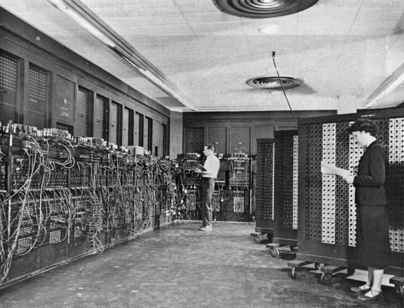
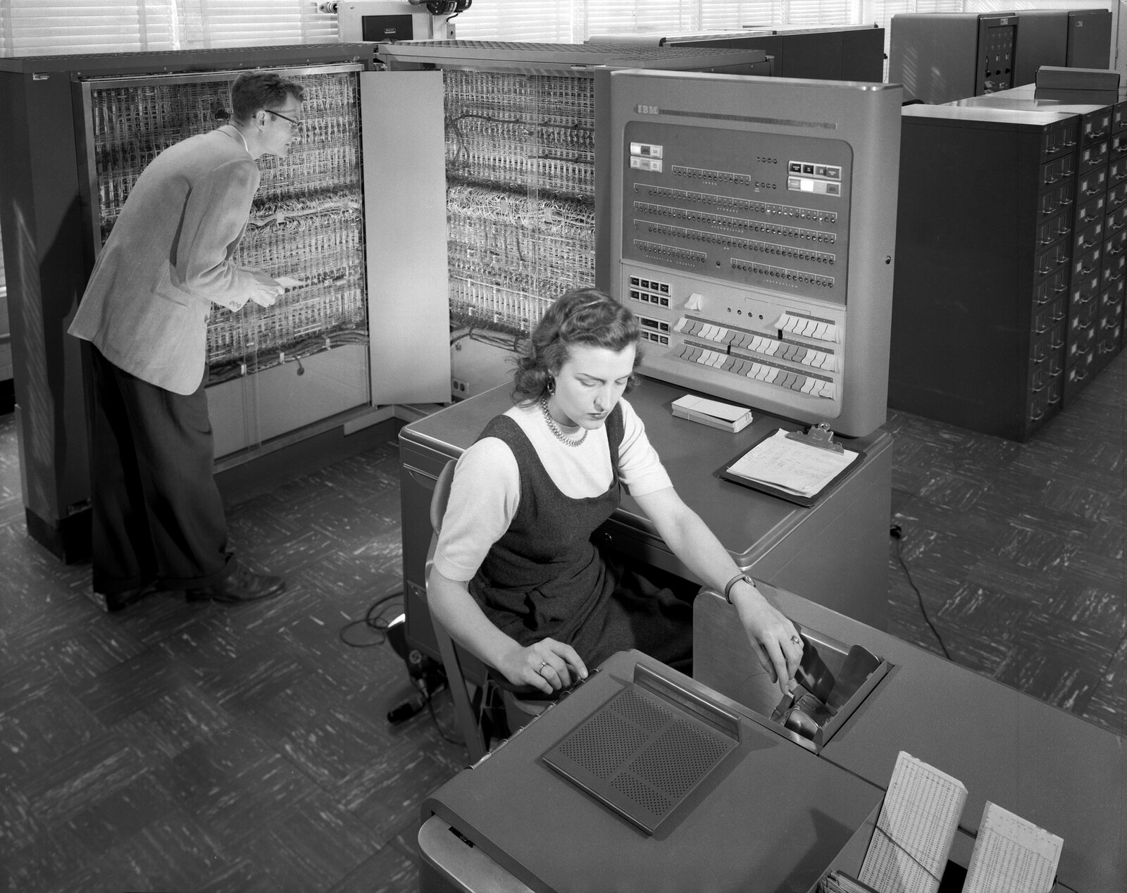
The Electronic Numerical Integrator and Computer was born from war. In 1943, the U.S. Army needed faster ballistic firing tables – each table required a human “computer” (usually a woman with a desk calculator) to spend 20 hours on a single trajectory. There was a backlog of firing tables. The gun crews at the front were shooting with less-than-optimal aim because the math hadn’t caught up.

John Mauchly, a physicist at the Moore School of Electrical Engineering at the University of Pennsylvania, had an idea: build an electronic calculator using vacuum tubes. He had been thinking about this since 1941, partly inspired by the Atanasoff-Berry Computer he had seen at Iowa State. His young graduate student J. Presper Eckert – a brilliant engineer with an almost obsessive attention to reliability – figured out how to actually make it work.

The Army said yes. Project PX began in June 1943. Budget: $61 700 for the first six months (it would eventually cost roughly half a million dollars).

What they built was staggering.

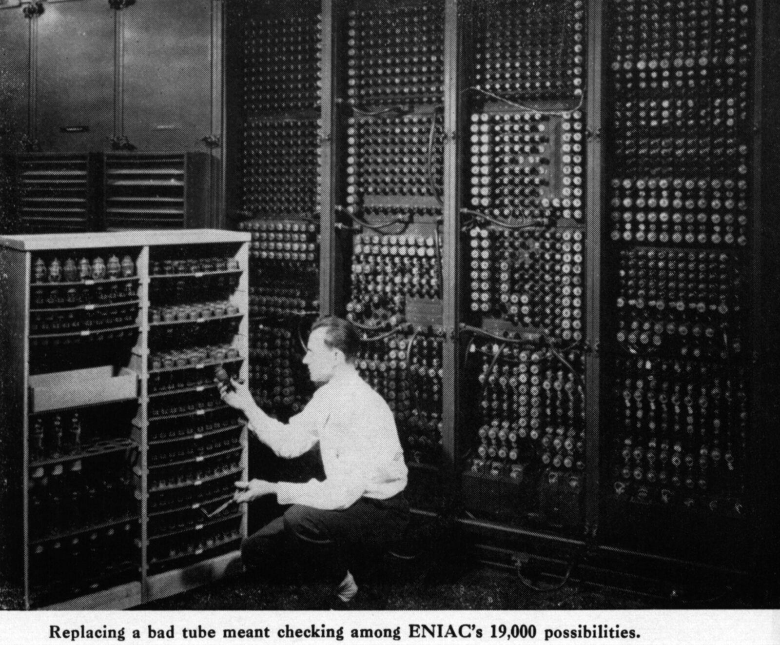
17 468 vacuum tubes. Each tube was a glass bottle about the size of your thumb, containing a heated filament in a vacuum. Electrons flew between electrodes inside the tube, switching on and off – the basic binary operation. But 17 468 of them? Vacuum tubes failed constantly. The engineering consensus at the time was that any machine with more than a few hundred tubes would be down more than it was up. Eckert’s genius was in running the tubes at lower-than-rated voltages and implementing rigorous quality control – reducing the failure rate from one tube per hour to one every two days.

70 000 resistors. 10 000 capacitors. 6 000 switches. 5 million hand-soldered joints. The machine filled a room the size of a tennis court – roughly 15 by 9 meters – arranged in 40 panels along three walls shaped like a U. It weighed 30 tons. It consumed 174 kilowatts of power and needed two 20-horsepower blowers and its own air conditioning system just to keep from melting.

And here’s the detail that gets lost in the spectacle: the ENIAC used decimal arithmetic, not binary. Each of its 20 “accumulators” stored a single 10-digit decimal number using ring counters – 10 vacuum tubes per digit, one tube on at a time to represent 0-9. This was a deliberate choice: Mauchly and Eckert wanted the machine to be compatible with the decimal world of engineering tables and human calculators. It worked, but it was spectacularly wasteful of tubes.

Programming = Physical Labor

I’ve told this part of the story before, but it bears repeating in the context of what came next.

There was no software. There was no programming language. There was no stored program. The ENIAC’s “program” was its physical wiring. To solve a different problem, you had to rewire the machine – routing data between the 40 panels by plugging and unplugging patch cables, setting thousands of switches to the right positions, consulting the machine’s blueprints to figure out which unit should feed into which.

Setting up a new problem could take days to weeks. Running the problem itself might take minutes or hours. Then you tore it all out and started over for the next problem.

The first people to do this – the original ENIAC programmers – were six women mathematicians: Kay McNulty, Jean Jennings, Betty Snyder, Marlyn Wescoff, Fran Bilas, and Ruth Lichterman. They had been computing ballistic trajectories by hand during the war. Now they were given the blueprints of the world’s first general-purpose electronic computer and told: figure out how to make it work. No manual. No precedent. No instructor. They invented the job of “programmer” – and their contributions went unrecognized for decades. The press photographed the machine, not the women standing in front of it.

The Weather and the Bomb

The ENIAC’s first calculations were not ballistic tables. They were hydrogen bomb simulations.

In the fall of 1945 – before the machine was even publicly unveiled – John von Neumann arranged for two physicists from Los Alamos to come to Philadelphia and run the first problem: a calculation related to the feasibility of a thermonuclear weapon. The two physicists were Nicholas Metropolis and Stan Frankel.

Remember that name. Stan Frankel. He will come back.

The H-bomb calculation ran for several weeks and consumed about a million punch cards. The result was classified. But the ENIAC had proved something: electronic computing could tackle problems that were far beyond human calculation speed.

Then came Monte Carlo methods. Stan Ulam, recovering from encephalitis in 1946, had the insight that random sampling could solve problems in neutron diffusion (how neutrons bounce around inside a nuclear weapon). He and Metropolis implemented it on the ENIAC. The method was named “Monte Carlo” after the casino, because Ulam’s uncle had a gambling habit. It is now one of the most widely used computational techniques in all of science – from particle physics to financial modeling to weather ensemble forecasting. Readers who have followed this series will recognize ensemble forecasting as Lorenz’s legacy made operational.

And then came the weather. In March 1950, readers of this series already know what happened: Charney, Fjortoft, and their team spent 33 days and nights at Aberdeen Proving Ground, cycling through 14 punch-card operations per time step, punching roughly 100 000 IBM cards, to produce the first numerical weather forecast. A 24-hour forecast in 24 hours. The barotropic vorticity equation, on a 19 × 16 grid, at 736 km spacing.

The actual ENIAC programming for the weather forecast was done by Klara Dan von Neumann – John von Neumann’s wife, a mathematician in her own right who had learned to code the ENIAC and checked the final program. Without her, the 100 000 punch cards would not have been in the right order.

The Person to Remember: Klara Dan von Neumann

Klara (born Klári Dán in Budapest, 1911) married John von Neumann in 1938. During the war, she was one of the first people to learn ENIAC programming. She coded the weather forecast program, she coded the H-bomb simulations, and she tested and debugged the code on a machine that had no debugger – just 17 468 vacuum tubes and a prayer.

She is rarely mentioned in histories of computing. When the Smithsonian wrote about the weather forecast, they called her “the computer scientist you should thank for your phone’s weather app.” That headline appeared in 2017 – sixty-seven years after the fact.

The Conversion: A Bridge Between Eras

In 1948, von Neumann and his colleagues Richard Clippinger and Adele Goldstine (Herman’s wife, another unsung mathematician) devised a way to make the ENIAC simulate a stored program. Instead of rewiring the machine for each new problem, they configured the patch cables into a fixed wiring that implemented a small set of general instructions – essentially turning the ENIAC into a simple stored-program machine. The program itself was stored on the function table switches (Haigh, Priestley & Rope, 2016).

The conversion worked, but at a cost: the rewired ENIAC was roughly six times slower than the original, because it now had to fetch and decode instructions rather than executing hardwired operations. But the trade-off was worth it. Reprogramming went from weeks to hours. The ENIAC in its converted form ran from 1948 until it was finally decommissioned on October 2, 1955, at 11:45 PM – a decade of continuous service.

This conversion was the conceptual bridge between the ENIAC and the IAS machine. Von Neumann had proved the stored-program concept could work, even on hardware not designed for it. Now he wanted to build a machine that was designed for it from the ground up.

What the ENIAC Changed

The ENIAC proved three things:

1. Electronic computing works. Despite the engineering consensus that a machine with thousands of vacuum tubes would be too unreliable, Eckert’s discipline – running tubes at 50-80% of rated voltage, testing every component before installation – made it run (Kleiman, 2022).
2. The atmosphere can be predicted by machine. Charney’s forecast wasn’t great. But three of the four cases beat persistence – predicting that tomorrow looks like today.¹ And Charney said the rest was “purely a technological problem.”²
3. Electronic computers could be converted from special-purpose to general-purpose. The 1948 stored-program conversion showed that the future lay in flexible, programmable machines – not hardwired calculators.

But even in its converted form, the ENIAC had a fatal limitation: its internal memory held only 20 numbers. Everything else lived on punch cards, shuttled in and out by operators. You couldn’t load a complex program into memory and let it run. You couldn’t iterate. You couldn’t explore.

For that, you needed a machine designed around a different principle entirely.

The Missing Link: EDVAC

Before the IAS machine, there was the EDVAC – the Electronic Discrete Variable Automatic Computer. Where the ENIAC was decimal, EDVAC was binary. Where the ENIAC stored its program in patch cables, EDVAC would store it in memory. Where the ENIAC used 17 468 vacuum tubes, EDVAC needed only about 3 500 – because binary arithmetic is inherently simpler than decimal.

Von Neumann laid out the EDVAC’s design in his famous “First Draft of a Report on the EDVAC” (June 1945) – the document that introduced the stored-program concept to the world. But here’s the irony: EDVAC itself was plagued by delays. Eckert and Mauchly left the Moore School in March 1946, bitter over patent disputes with von Neumann. The remaining team struggled. Construction dragged on for years.

EDVAC’s memory was another innovation: mercury delay lines. The idea was almost absurdly physical – electrical signals were converted to sound pulses, sent through a tube filled with liquid mercury, received at the other end, converted back to electrical signals, and recirculated in a loop. Data literally traveled as sound waves through heavy metal. Each tube was about five feet long and held roughly 1 000 bits. It worked, but it was slow (serial access only) and required precise temperature control – the speed of sound in mercury changes with temperature.

By the time EDVAC finally became operational at Aberdeen in 1951, other machines inspired by its design had already beaten it into service. Most famously, EDSAC at Cambridge University (built by Maurice Wilkes) ran its first program on May 6, 1949 – becoming the first practical stored-program computer in the world. Wilkes had attended the Moore School Lectures in the summer of 1946, gone home to England, and built his own version faster than the original team could finish theirs.

EDVAC served at Aberdeen from 1951 to 1962, running ballistic calculations and military research. It never achieved the fame of the ENIAC or the IAS machine. But its design – binary, stored-program, with instructions and data sharing the same memory – was the template for everything that followed. Von Neumann took those principles and built the IAS machine. And the IAS machine changed the world.

---

Machine 2: The IAS Machine – The Architecture (1952)

Von Neumann’s Idea

John von Neumann saw the ENIAC being programmed and realized something that would reshape all of computing.

If the program was just a pattern of instructions, and the data was just a pattern of numbers, then both could live in the same memory. The program could be stored alongside the data and modified during execution. No more rewiring. No more patch cables. You change the program by changing numbers in memory.

This idea – the stored-program concept – appeared in von Neumann’s “First Draft of a Report on the EDVAC” in June 1945. The report was written in von Neumann’s name alone, which caused a bitter dispute with Eckert and Mauchly, who argued they had discussed the concept first. The debate has never been fully resolved. But regardless of priority, it was von Neumann who formalized the architecture and, crucially, decided to publish it openly.

That openness changed everything.

Building the Machine

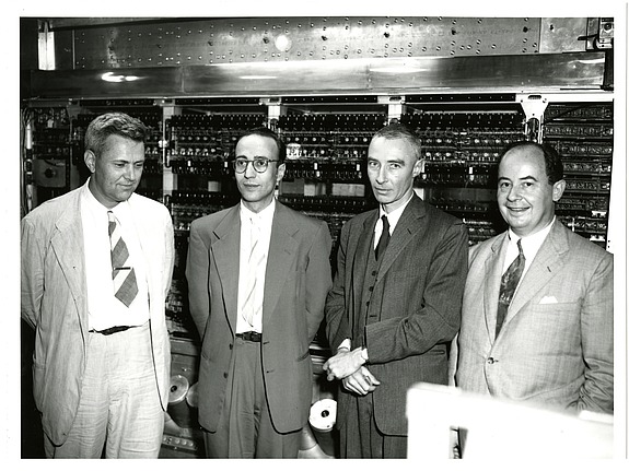
Von Neumann returned to the Institute for Advanced Study in Princeton – the same institute where Einstein had an office – and proposed building a computer. The IAS board was skeptical. A calculating machine at an institute for pure mathematics? Von Neumann argued that computing was applied mathematics of the highest order, and that the machine would be used for problems of fundamental scientific importance: hydrogen weapons, meteorology, fluid dynamics, and even biology.

The board approved the project. Julian Bigelow, a young MIT-trained engineer who had worked on anti-aircraft fire control during the war, was hired as chief engineer. Herman Goldstine, a mathematician who had been the Army’s liaison to the ENIAC project, joined as the project’s administrative and intellectual bridge between von Neumann’s vision and the engineering reality.

Construction began in 1946. It took six years – much longer than planned. The machine was first operational in 1951 and publicly demonstrated on June 10, 1952.

5 Kilobytes of Lightning

The IAS machine’s memory was its most revolutionary and most temperamental component: Williams tubes – cathode-ray tubes used as memory.

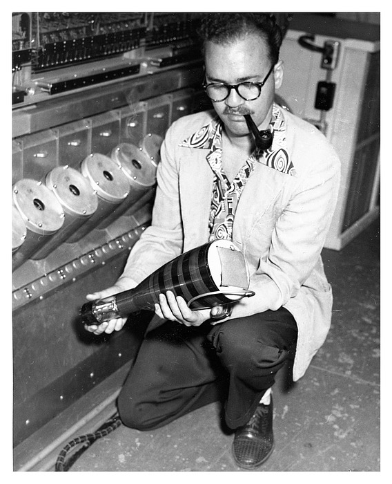
Here’s how they worked. A cathode-ray tube (the same technology as an old television screen) shoots a beam of electrons at a phosphorescent screen. When the beam hits a spot, it leaves a small electric charge. By directing the beam to specific locations and reading back the charge, you can store and retrieve binary digits (Williams & Kilburn, 1949).

The IAS machine had 40 Williams tubes, each storing 1 024 bits (organized as 32 rows of 32 bits). Total: 40 960 bits, or 1 024 words of 40 bits each – roughly 5 kilobytes.

It was elegant. It was fast (access time measured in microseconds, not the milliseconds of drum-based memory). And it was horrifically unreliable. The charges faded. Static electricity interfered. Temperature changes caused drift. The tubes had to be recalibrated constantly. Engineers spent as much time nursing the memory as scientists spent running programs.

Phillips, who ran his general circulation experiment on this machine, described the programming experience in terms that would make a modern developer weep:

“Code was written in what would now be called ‘machine language’ except that it was one step lower – the 40 bits of an instruction word (two instructions) were written by us in a 16-character (hexadecimal) alphabet.”³

No compiler. No assembler. No DO-loops. Raw hexadecimal, hand-coded. Each instruction was a pattern of hex digits specifying an operation code and a memory address. If you wanted a loop, you wrote the loop counter explicitly. If you wanted a subroutine, you manually stored the return address.

On this machine. In 5 kilobytes.

Not Just Weather: Artificial Life on 5 Kilobytes

Before Phillips ran his climate experiment, the IAS machine had already hosted something even more speculative. In 1953, an Italian-Norwegian mathematician named Nils Aall Barricelli used the machine to run what may have been the first artificial life simulations in history.

Barricelli created a one-dimensional universe of numbers on the machine’s memory, gave them rules for reproduction and mutation, and watched them evolve. He observed parasitism, symbiosis, and something that looked disturbingly like natural selection – digital organisms competing for memory space (Dyson, 2012). His work was published in obscure journals and largely ignored for decades. It anticipated genetic algorithms and artificial life research by thirty years.

Von Neumann himself was fascinated by the connection between computing and biology. His last major intellectual project, unfinished at his death, was a theory of self-reproducing automata – machines that could build copies of themselves. The IAS machine was where that theory was meant to be tested.

The same 5 kilobytes that simulated the atmosphere also simulated evolution. The machine didn’t care what the numbers meant.

The Science: The First Climate Model

In 1955-56, Norman Phillips – readers who follow this series already know him – used the IAS machine to run the first general circulation experiment. Starting from an atmosphere at rest, with nothing but simple differential heating, his two-layer model produced jet streams, surface wind patterns, a realistic cyclone, and fronts. From 500 variables (Phillips, 1956).

I’ve told that story already. What I haven’t told you is how the machine’s limitations shaped the experiment.

Phillips’ entire model – the atmospheric state, the program code, everything – had to fit in 1 024 words of memory. His atmosphere was described by roughly 500 numbers. The program occupied the rest. There was no room for a more complex model even if he had wanted one. The two-layer, 17 × 16 grid wasn’t just a scientific choice. It was the maximum the hardware could hold.

The IAS machine’s drum memory (an auxiliary storage device, slower than the Williams tubes but more reliable) held 2 048 words initially, later upgraded to 16 384. Phillips used it for intermediate results that wouldn’t fit in main memory. Every drum access meant waiting for the cylinder to rotate to the right position – slowing the calculation by orders of magnitude compared to a pure Williams-tube computation.

The 31 simulated days of Phillips’ experiment took 11 to 12 hours on the IAS machine.

The Clones: Open Source Before the Term Existed

Here’s the most extraordinary thing von Neumann did. He published the complete design of the IAS machine – blueprints, circuit diagrams, engineering reports – and made them freely available to anyone who wanted to build a copy.

No patents. No licenses. No fees.

This was a deliberate philosophical choice. Von Neumann believed that computing was too important to be locked behind intellectual property. (His attitude toward the bomb patents was rather different, but that’s another story.) The result was an explosion of IAS clones – machines built to the same design at labs and universities around the world:

• MANIAC – Los Alamos National Laboratory. Built by Metropolis (the same Metropolis who had run the H-bomb calculations on the ENIAC). Used for weapons simulations.
• JOHNNIAC – RAND Corporation, Santa Monica. Named after von Neumann (Johnny). Used for military research and, eventually, the first experiments in artificial intelligence.
• ILLIAC – University of Illinois. Used for research across physics, chemistry, and music (the Illiac Suite of 1957 was one of the first pieces of music composed by a computer).
• ORDVAC – Aberdeen Proving Ground. Built for the Army. Replaced the ENIAC for ballistic calculations.
• WEIZAC – Weizmann Institute of Science, Israel. The first computer in the Middle East. Von Neumann personally helped the Israeli team.
• SILLIAC – University of Sydney, Australia. Named with characteristic Australian irreverence.
• BESM – Moscow. The Soviet Union built their own version, drawing on the published IAS design. Computing, like physics, respects no borders.

Each clone was slightly different – tweaked for local needs, improved by local engineers. But they all descended from von Neumann’s architecture. They all stored their programs in memory. They all used binary arithmetic. They all spoke the same fundamental language.

This was the birth of the modern computer. Not one machine, but an architecture – replicated, adapted, and improved across the world. Every computer you have ever used, from the mainframe in your bank to the phone in your pocket, descends from the design von Neumann published and gave away for free.

The Person to Remember: Julian Bigelow

Von Neumann gets the credit. And he deserves much of it – his mathematical insight was essential. But the person who actually built the IAS machine was Julian Bigelow.

Bigelow was 32 when he joined the project in 1946. He had been working on Norbert Wiener’s anti-aircraft predictor at MIT – the same project that gave rise to cybernetics. He was, by all accounts, a quiet, meticulous, deeply practical engineer. Von Neumann would outline what the machine needed to do. Bigelow would figure out how to make the physics actually work – how to wire the tubes, how to stabilize the Williams tube memory, how to get thousands of components to function together reliably enough to run for hours without crashing.

He has no Wikipedia article as of this writing. His name appears in footnotes.

What the IAS Machine Changed

1. The stored-program concept became real. Programs lived in memory. You could change what the computer did by changing numbers, not cables.
2. Computing became replicable. The published design spawned clones on every continent. No longer one machine in one room – an architecture available to anyone willing to build it.
3. Climate science was born. Phillips’ experiment proved that the atmosphere could be simulated from first principles. That led directly to GFDL, to Manabe, and eventually to a Nobel Prize.

But the IAS machine was still a one-off research instrument, hand-built by engineers at a research institute. You couldn’t buy one. You couldn’t order a spare part. If a Williams tube failed at 2 AM, you woke up the engineer.

Computing needed to become a product.

---

Machine 3: The IBM 700 Series – The Factory (1952-1956)

Computing Goes Commercial

In the early 1950s, a question hung over the computing world: was this a curiosity for government labs, or was there a real market?

IBM answered it.

The IBM 701, announced in April 1952 and delivered from December of that year, was IBM’s first commercial scientific computer. It was designed under Nathaniel Rochester, who had previously designed radar systems at MIT. The 701 used electrostatic memory (Williams tubes, like the IAS machine) and could perform about 16 000 additions per second. It cost roughly $15 000 per month to rent – IBM didn’t sell, they leased – and it was built to a production standard. If something broke, IBM sent a technician. If you needed a manual, IBM printed one.

IBM expected to sell five units. They got eighteen orders. (This is the real story behind the famous misquote “I think there is a world market for maybe five computers,” which I’ve debunked before.)

But the 701 still had the Williams tube problem – unreliable, temperamental, prone to data loss. What computing needed was a memory technology that worked.

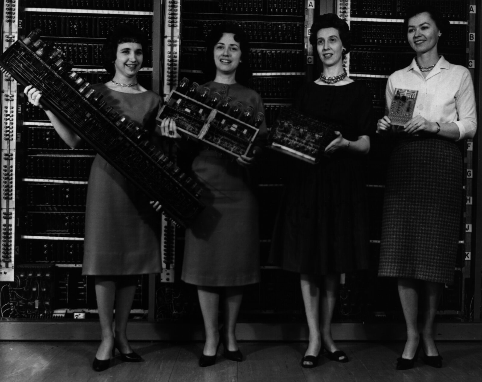
Jay Forrester’s Tiny Rings

The breakthrough came from MIT – not from the computing group, but from Project Whirlwind, a real-time flight simulator originally designed for the Navy.

Jay Forrester, the project leader, needed memory that was fast, reliable, and non-volatile (meaning it wouldn’t lose data when the power flickered). Williams tubes were none of these things reliably. The Whirlwind computer was intended for real-time applications – if the memory glitched during a flight simulation, the virtual airplane crashed. Unreliable memory was not an inconvenience. It was a showstopper.

In 1949, Forrester had the idea that would dominate computer memory for two decades: magnetic core memory (Forrester, 1951).

The concept was deceptively simple. Take a tiny ring of ferrite (iron-based ceramic), about 1 millimeter in diameter. Thread wires through it. Run a current through the wires, and the ring magnetizes in one direction (representing a 1) or the other (representing a 0). The magnetization persists with no power – non-volatile. Reading the core is destructive (you have to flip the magnetization to detect it, then write it back), but it’s fast and utterly reliable.

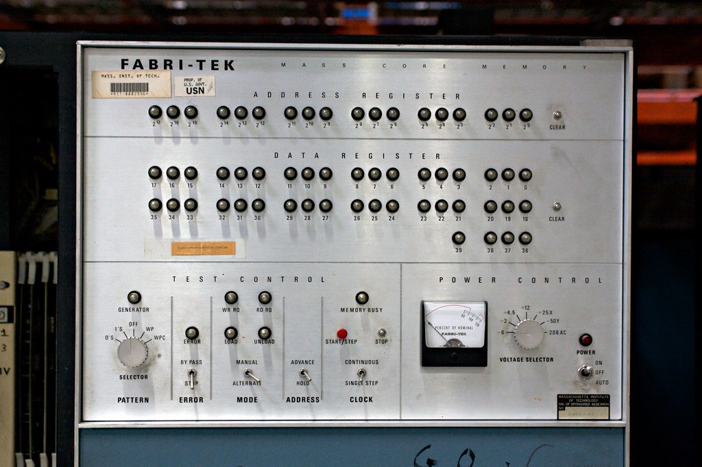
The engineering challenge was scale. Each bit of memory required one tiny ferrite core. Each core had to be threaded onto a grid of wires – three or four wires per core, woven through by hand. A memory plane of 1 024 bits required 1 024 cores and thousands of wire-threading operations.

This work was done almost entirely by women – at MIT, at IBM, at every manufacturer. They sat at tables with magnifying glasses and fine needles, threading hair-thin copper wire through rings the size of pinheads, row after row, plane after plane. The work was called core rope manufacturing. It required extraordinary patience and dexterity. A single memory module of 32 768 words (the IBM 704’s full memory) contained over a million individual cores, each hand-threaded.

The women who built these memory planes are almost entirely unnamed in the historical record.

The IBM 704: Memory, Math, and a New Language

The IBM 704, which shipped in late 1955, was the first mass-produced computer to incorporate both magnetic core memory and hardware floating-point arithmetic.

The specs represented a leap:

• Memory: 32 768 words of 36 bits each – roughly 144 kilobytes. Core memory. Fast. Reliable. No more Williams tube crashes.
• Speed: About 40 000 fixed-point additions per second. 12 000 floating-point operations per second.
• Floating point in hardware: Previous machines (including the ENIAC and IAS) had to simulate floating-point arithmetic in software – a slow, tedious process. The 704 had dedicated circuitry for it. For scientific computing, this was transformative.
• Cost: About $2 million to purchase, or roughly $32 000 per month to lease.
• Production: About 123 units were sold. A real production run, not a one-off.

The chief architect was Gene Amdahl, a young engineer who would later formulate Amdahl’s Law – the observation that the speedup of a program from parallelization is limited by the fraction of the program that cannot be parallelized. Every person who has ever tried to speed up a weather model by throwing more cores at it has cursed Amdahl’s name. (He also, later, left IBM and founded his own competing mainframe company. IBM was not amused.)

But the 704’s most important contribution wasn’t hardware. It was a language.

FORTRAN: The Revolution You Take for Granted

In 1953, John Backus, a 29-year-old programmer at IBM, sent a memo to his manager proposing the development of a “FORmula TRANslation” system for the 704. The idea: let scientists write mathematical formulas in something close to normal notation, and have the computer translate those formulas into machine code automatically.

This was heresy.

The prevailing belief in the 1950s was that no automatic translation system could produce code as efficient as what a skilled human programmer could write by hand. Machine code was sacred. Assembly language (a thin layer over machine code) was considered the height of convenience. A “high-level” language would waste the machine’s precious cycles.

Backus and his team of about ten programmers spent three years on it. The first FORTRAN compiler was delivered with the IBM 704 in April 1957. It was 25 000 lines of machine code and could compile a FORTRAN program into machine instructions that ran within 20% of the speed of hand-coded programs. For most users, the difference was invisible.

The effect was immediate and total. Within a year, more than half of all code written for the 704 was in FORTRAN. Within a decade, FORTRAN was the universal language of scientific computing.

Think about what this meant for atmospheric science. Before FORTRAN, every weather model was written in machine code or assembly language. Every meteorologist who wanted to run a numerical experiment needed to think like a computer engineer – worrying about memory addresses, register allocation, instruction sequences. Phillips coded his general circulation model in hexadecimal, by hand, one instruction at a time.

After FORTRAN, a meteorologist could write:

      DO 100 I = 1, NLON
      DO 100 J = 1, NLAT
        TEMP(I,J) = TEMP(I,J) + DT * HEATING(J)
  100 CONTINUE

That’s a double loop updating temperature across a latitude-longitude grid. The FORTRAN compiler would turn this into the right sequence of machine instructions for the 704. The scientist could focus on the physics, not the plumbing.

FORTRAN didn’t just make programming easier. It made a new generation of atmospheric scientists possible – people who understood the atmosphere but didn’t need to understand the inner workings of the hardware. The language separated the science from the machine.

And it’s still here. The ECMWF’s Integrated Forecasting System, the model that produces the best weather forecasts on Earth, is written in FORTRAN. Updated, modernized, ported through dozens of hardware generations – but FORTRAN. Seventy years later.

The Science: Weather Prediction Becomes Routine

In my Charney post, I mentioned that the Joint Numerical Weather Prediction Unit (JNWPU) was established in 1954 in Suitland, Maryland. An IBM 701 was installed in March 1955, and by May of that year, the first routine real-time operational numerical weather forecasts in the United States began.

But were the Americans really first? Rossby had returned to Stockholm. He had access to a computer. And he was not the kind of man who waited for someone else to go first. More on that soon.

It was the IBM 704 that turned American operational NWP from a struggle into a system. With 144 kilobytes of reliable core memory, hardware floating point, and eventually FORTRAN, the JNWPU could run more complex models, add more vertical levels, increase the resolution, and – crucially – run twice daily on a schedule that never slipped.

By 1958, the IBM 704 at the JNWPU was producing operational forecasts using Charney’s three-level quasi-geostrophic model. The forecasts were good enough that the U.S. Weather Bureau began distributing them to field offices. Weather prediction by computer was no longer an experiment. It was infrastructure.

The 704 also ran the first serious experiments in tropical cyclone forecasting, the first attempts at statistical weather prediction (using past weather patterns rather than physical equations), and the earliest work on spectral methods (representing atmospheric fields as sums of mathematical waves rather than values on a grid). All of these would become pillars of modern NWP.

And because the 704 ran FORTRAN, the code could be shared. A model developed at one institution could be compiled and run at another. The research community could collaborate in ways that machine-code programming made nearly impossible. Open science, enabled by a programming language.

The IBM 704 Beyond Weather

The 704 was also where John McCarthy implemented Lisp in 1958 – the second-oldest high-level programming language still in use (after FORTRAN). Lisp became the language of artificial intelligence research for three decades.

At Bell Labs, Max Mathews created the MUSIC program on the IBM 704 in 1957 – the first software for digital audio synthesis. His work led to the famous 1961 recording of “Daisy Bell” (also known as “A Bicycle Built for Two”), performed on the IBM 7094 with vocals synthesized by John Kelly’s speech program and accompaniment by Mathews’ MUSIC IV. When Stanley Kubrick needed the HAL 9000 computer to sing a song as it was being shut down in 2001: A Space Odyssey (1968), he chose “Daisy Bell” – Arthur C. Clarke had visited Bell Labs and heard the 7094 sing it in person.

The People to Remember

John Backus gave us FORTRAN. He later contributed to Algol (the ancestor of C, Java, and most modern languages) and spent his later career arguing that the von Neumann architecture was fundamentally limiting – a position he laid out in his 1977 Turing Award lecture, “Can Programming Be Liberated from the von Neumann Style?”

Jay Forrester gave us core memory. He later became a pioneer of system dynamics – the discipline of modeling complex systems with feedback loops. His 1971 book World Dynamics was one of the first computer simulations of global population, pollution, and resource depletion. A man who built computer memory went on to model the memory of the planet.

Gene Amdahl gave us the 704’s architecture and the law that bears his name. Any time a weather center debates whether to buy a faster computer or a wider one (more cores vs. faster cores), they’re working within the framework Amdahl described in 1967.

And the unnamed women who threaded a million ferrite cores by hand gave us the memory that made it all reliable.

What the IBM 700 Series Changed

1. Computing became a product. You could order a computer from a catalog. IBM sent a manual and a technician. The era of one-off, hand-built research machines was ending.
2. Core memory made computing reliable. No more Williams tube crashes. The data stayed put.
3. FORTRAN made computing accessible. Scientists could write physics, not machine code.
4. NWP became operational. Weather forecasting by computer went from a heroic experiment to a daily routine.

But the IBM 704 cost two million dollars, filled a room, and required a staff of operators. If you were a lone scientist at a university – say, a quiet meteorologist at MIT who wanted to explore an atmospheric model at his own pace – you were out of luck. You submitted your job to the computing center, waited hours or days for results, picked up a printout, and if something was wrong, started over.

You couldn’t sit next to the machine and watch it think.

For that, you needed a desk.

---

Machine 4: The LGP-30 – The Desk That Discovered Chaos (1956)

The Man Who Built It

This is the thread that runs through the entire story, and almost nobody tells it.

Stan Frankel was a physicist. In the early 1940s, he was at Los Alamos, working on the Manhattan Project. He was part of the T-Division – the theoretical physics group – alongside Hans Bethe, Edward Teller, and Richard Feynman. (Feynman later recalled Frankel as one of the people he worked with on setting up computation systems at Los Alamos, using rooms full of people with mechanical calculators arranged into human computing chains – Richardson’s forecast factory, built in a desert for a different purpose.)

In the fall of 1945, Frankel and Nicholas Metropolis traveled to Philadelphia to run the first calculations on the ENIAC – the hydrogen bomb feasibility study. Frankel was one of the first people in the world to program the ENIAC, albeit in the cable-and-switch sense of “program.”

He saw what the ENIAC could do. And he saw what it couldn’t – it was huge, expensive, and the province of governments and large research institutions. Ordinary scientists couldn’t get near it.

After the war, Frankel went to work at Librascope, a division of General Precision Equipment Corporation in Glendale, California. Librascope made precision instruments – optical devices, navigation equipment, things that needed careful engineering. Frankel proposed building a computer. Not a giant. Not a room-filler. Something a scientist could have in their office.

113 Tubes and a Spinning Drum

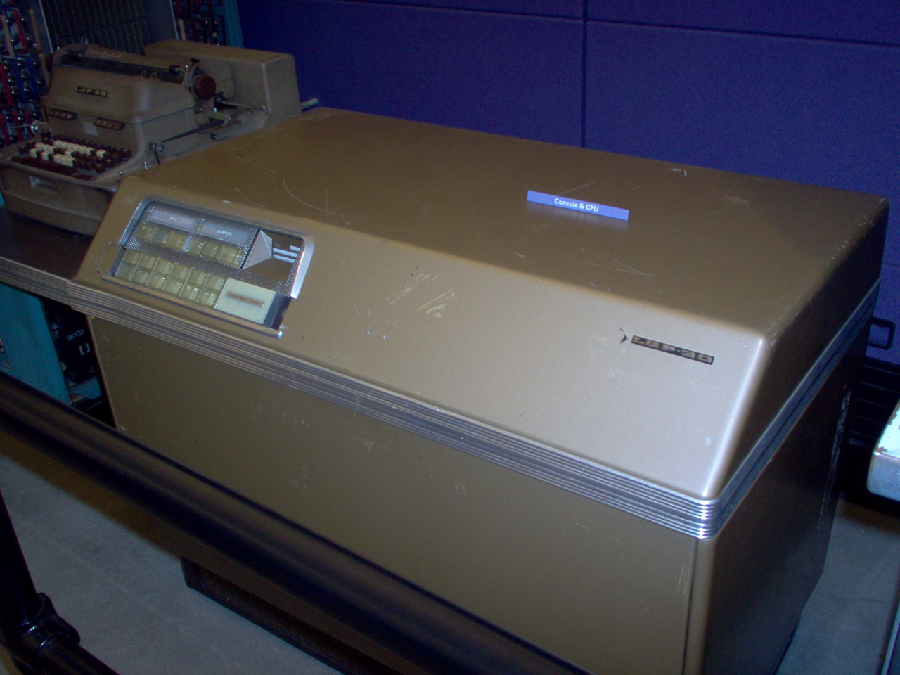
The Librascope General Purpose computer, 30-bit word length – the LGP-30 – was Frankel’s answer to a question nobody else was asking: what if computing was personal?

The design was a masterpiece of minimalism. Where the ENIAC used 17 468 vacuum tubes, the LGP-30 used 113. Where the IAS machine used fragile Williams tubes for memory, the LGP-30 used a magnetic drum – a solid metal cylinder about 6.5 inches in diameter, spinning at 3 700 rpm, with magnetic tracks on its surface. Where the IBM 704 used core memory hand-threaded by women, the LGP-30 stored everything on the drum: 4 096 words of 31 bits each, about 16 kilobytes.

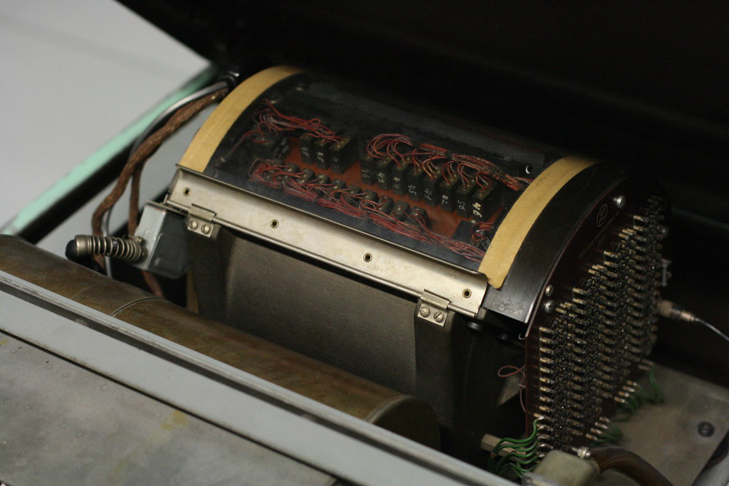
The drum was the key cost-saving trick. Core memory was fast but expensive. Williams tubes were fast but unreliable. The drum was slow but cheap and nearly indestructible. Data was read by waiting for the right spot on the spinning surface to pass under a read head – which meant the effective speed of the machine was limited by the drum’s rotation rate. The 120 kHz clock could, in theory, execute instructions quickly, but most of the time was spent waiting for the drum.

Result: about 60 operations per second. Roughly a thousand times slower than the IBM 704.

Expert programmers could squeeze more speed out of the drum through a technique called optimum programming (also called minimum-access coding). The trick was to arrange instructions on the drum surface so that by the time the processor finished executing one instruction, the drum had rotated to exactly the right position for the next one. Getting this right required thinking about the physical geometry of a spinning cylinder while writing code – a fusion of programming and mechanical engineering that has no modern equivalent. A well-optimized program could run five to ten times faster than a naively written one (Frankel, 1956). Lorenz, a meteorologist and not a systems programmer, almost certainly did not bother. His programs ran at whatever speed the drum allowed.

But the price.

$47 000. In 1956 dollars, that’s roughly $560 000 today. Sounds like a lot? The IBM 704 cost $2 million. The ENIAC had cost half a million in 1945 dollars. No individual scientist was writing a personal cheque for an LGP-30 – at $47 000, it was still a major capital purchase. But here’s the difference that mattered: a university department could afford one. The meteorology department. The physics department. A small engineering firm. These were buyers who could never have justified an IBM 704, let alone the staff to operate one.

The machine sat on sturdy casters. It weighed 800 pounds – heavy, yes, but not “structural-engineer-required” heavy. It ran on a standard 110-volt wall outlet. No special power supply. No air conditioning system. No raised floor. No dedicated room. A department bought it, rolled it into a professor’s office, plugged it in – and from that point on, the professor was the computing center. No operators. No batch queue. No waiting.

In Lorenz’s case, the MIT Department of Meteorology purchased the LGP-30 and installed it in his office. He was, for all practical purposes, the sole user. The machine was institutional property, but the experience of using it was personal – one scientist, one machine, no intermediaries. That distinction between who owned the computer and who used the computer is the whole revolution.

About 500 units were sold – to universities, government labs, small companies, and engineering firms across North America and Europe. For the era, that was a hit. The IBM 704 sold 123 units. The LGP-30 outsold it four to one, because departments that could never afford a mainframe could afford a desk.

The Flexowriter: Computing You Can Hear

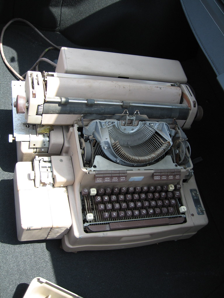
The LGP-30’s input and output device was a Friden Flexowriter – a modified electric typewriter that could read and punch paper tape and print characters on paper. It was the keyboard, the printer, and the storage medium, all in one clattering machine.

This created something entirely new: interactive computing. You typed a command. The Flexowriter clacked. The drum spun. Numbers appeared on the paper. You saw the result immediately. If it looked wrong, you stopped the program. If it looked interesting, you let it run.

On an IBM 704, you submitted your job as a deck of punch cards, waited for the operators to load it, waited for the machine to run it between other people’s jobs, and picked up your printout hours or days later. On the LGP-30, the machine was yours. You were the operator. You sat in front of it, watched the numbers print, heard the drum spin, and followed your calculation in real time.

This difference is not trivial. It is the difference between batch processing (submit, wait, collect results) and exploration (try, observe, think, try again). The batch model is efficient for running known programs. The exploration model is how you discover things you didn’t expect.

And that is exactly what happened.

The Science: One Cup of Coffee

In the winter of 1961, a quiet meteorologist at MIT named Edward Lorenz was running a simplified weather model on the LGP-30 installed in his office. Readers of this series already know the story – the restarted run, the truncated decimals, the diverging outputs, the discovery that deterministic systems can be unpredictable.

But here’s what I didn’t emphasize before: the discovery required the LGP-30’s specific combination of features.

1. It was in Lorenz’s office. He could watch the output scroll line by line. On a shared mainframe, he would have received a printout and compared it to another printout – a static comparison, easy to dismiss as a computational error. On the LGP-30, he watched the divergence happen in real time, line by clacking line. He could see the weather pattern evolving, see it start to differ, see it drift further and further. The visual unfolding is what made the discrepancy unmistakable.

2. It was slow enough to restart mid-run. The LGP-30 did about 60 operations per second. Lorenz’s model printed a new line – one time step – roughly every minute. A full run took hours. If the machine had been fast (like the IBM 704), a complete run would have taken minutes, and there would have been no reason to restart from the middle. The slowness of the drum made the shortcut rational.

3. The printout showed fewer digits than the internal state. The Flexowriter printed three decimal places. The drum stored six. This is the rounding that created the 0.000127 difference that changed science. A different I/O system – one that printed all six digits – would have eliminated the discrepancy entirely. Lorenz would have typed in the full-precision numbers, gotten the same result, and discovered nothing.

4. He could stop, think, and restart. The LGP-30 was his machine. Nobody was waiting for their batch job. He could let the coffee get cold. He could stare at the printout. He could go back, try again, change things. The machine accommodated the pace of human thought, not the schedule of a computing center.

The LGP-30’s limitations – its slowness, its low-precision printout, its presence in a single scientist’s office – were not obstacles to the discovery of chaos. They were preconditions for it.

From LGP-30 to LGP-21: The Transistor Revolution

Lorenz later upgraded to the Royal McBee RPC-4000, a transistorized machine in the same lineage. By the early 1960s, the vacuum tube was dying. Transistors – small, reliable, cool-running semiconductor devices – had replaced tubes in almost every application. The LGP-30 was one of the last successful vacuum tube computers. Its transistorized successors (the LGP-21, which cost just $16 200) were smaller, lighter, cheaper, and more reliable.

Stan Frankel designed those too.

Oh, and the name “Royal McBee” on Lorenz’s machine? Librascope was acquired by Royal McBee, which was a typewriter company. A typewriter company sold the computer that discovered one of the most important principles in all of physics. The universe has a sense of humor.

The Person to Remember: Stan Frankel

Frankel’s career traces the entire arc of this story. He computed nuclear weapon physics at Los Alamos with Feynman and Metropolis. He helped program the ENIAC for its very first problem. He designed the LGP-30 – the machine that put computing into individual scientists’ offices. And through that machine, he enabled Lorenz’s discovery of deterministic chaos.

He never became famous. He isn’t in the Computing Hall of Fame. He has no major prize named after him. But the thread from the Manhattan Project to chaos theory runs directly through Stan Frankel’s engineering choices – the decision to use a cheap drum instead of expensive core memory, the decision to build a minimal machine with 113 tubes instead of thousands, the decision to price it so that a university department could afford one.

Those choices put a computer on Lorenz’s desk. And Lorenz went for coffee.

What the LGP-30 Changed

1. Computing became personal in practice, if not in ownership. One scientist, one machine, in one office. The department bought it, but the scientist used it – alone, at their own pace, on their own questions. The experience of personal computing didn’t start in a Silicon Valley garage in the 1970s. It started when departments bought desk-sized machines and rolled them into professors’ offices.
2. Interactive exploration became possible. Batch processing gives you answers to questions you already know how to ask. Interactive computing lets you discover questions you didn’t know existed.
3. Chaos theory was born. Not from a billion-dollar supercomputer. From a $47 000 desk that did 60 operations per second.

---

The Arc

Let me put the four machines side by side one more time, but differently. Not by specs. By what they made possible.

ENIAC (1945): Proved that the atmosphere could be predicted by machine. Required a team, a building, and 33 days. The era of proving it could be done.

IAS Machine (1952): Proved that the atmosphere could be simulated from first principles – not just forecasted from today’s observations, but generated from nothing. Required a research institute and years of engineering. The era of understanding the climate.

IBM 704 (1955): Made weather prediction a daily operational reality. Required a computing center and a budget, but the models could be written in FORTRAN, shared, improved, and run on a schedule. The era of routine forecasting.

LGP-30 (1956): Revealed that weather prediction has a fundamental limit – not from lack of computing power, but from the mathematics of the atmosphere itself. Required nothing but a quiet scientist and an 800-pound desk. The era of discovering the boundaries.

Four machines. Four revolutions. Twenty years.

The Thread of People

There’s a human thread winding through all four machines, and it’s worth pulling together:

John von Neumann connected three of the four. He suggested the ENIAC’s first calculations. He designed the IAS machine’s architecture and published it for free. He organized the conference that led to GFDL. He influenced the IBM 700 series through the stored-program concept. He died of cancer in 1957, at 53, before most of the science his machines enabled had reached maturity. A security guard sat outside his hospital room at Walter Reed – even dying, von Neumann was considered a national security asset because of what he knew.

Stan Frankel connected the ENIAC to the LGP-30. He ran the first problem on the world’s first general-purpose electronic computer, then built the desk-sized computer that discovered chaos. From the largest to the smallest. From nuclear weapons to butterfly wings.

Klara Dan von Neumann wrote the actual programs – for both the H-bomb simulations and the weather forecast. The code that made the ENIAC useful for atmospheric science was hers.

Julian Bigelow built the IAS machine that von Neumann designed. Without Bigelow’s engineering, the stored-program concept would have remained a concept.

John Backus gave scientists a language to think in. FORTRAN freed meteorologists from machine code and allowed atmospheric science to scale.

Jay Forrester gave computers a reliable memory. Core memory ended the era of Williams tube crashes and made operational computing possible.

And the unnamed women – the six ENIAC programmers, the core rope threaders, the human computers of Los Alamos and Aberdeen – did the physical work that held the entire enterprise together, in an era that declined to record their names.

From 30 Tons to an 800-Pound Desk

The progression is staggering.

In 1945, predicting the weather required a machine that weighed 30 tons, consumed enough power to light a neighborhood, and needed a team of specialists to operate. The forecast took 24 hours to compute 24 hours ahead. One forecast. One level of the atmosphere. 19 × 16 grid points. Barely keeping pace with the weather.

In 1956 – eleven years later – a quiet man sat at an 800-pound desk plugged into a wall outlet, watched numbers clack out one line per minute, and discovered that weather prediction has a mathematical ceiling that no amount of computing power will ever break through.

The machines got smaller. The science got bigger.

And on my own desk, seven Raspberry Pi CM5s push 0.54 TFLOPS – roughly 9×10⁹ times faster than Lorenz’s LGP-30. Richardson’s 64 000 human computers, the ENIAC, the IAS machine, the IBM 704, the LGP-30, the Cray supercomputers, the massively parallel clusters – all of them compressed into a box with a Noctua fan.

But the two-week wall is still standing.

Lorenz proved it would always be standing.

With 60 operations per second.

---

Footnotes

---

References

ENIAC:

• Goldstine, H. H. (1972). The Computer from Pascal to von Neumann. Princeton University Press. WorldCat
• Kleiman, K. (2022). Proving Ground: The Untold Story of the Six Women Who Programmed the World’s First Modern Computer. Grand Central Publishing. Publisher
• Haigh, T., Priestley, M. & Rope, C. (2016). ENIAC in Action: Making and Remaking the Modern Computer. MIT Press. Publisher
• Metropolis, N. & Nelson, E. C. (1982). Early Computing at Los Alamos. Annals of the History of Computing, 4(4), 348-357. DOI
• Platzman, G. W. (1979). The ENIAC Computations of 1950 – Gateway to Numerical Weather Prediction. Bull. Amer. Meteor. Soc., 60(4), 302-312. PDF
• Encyclopaedia Britannica. ENIAC
• Army Ordnance Corps. Electronic Computers Within The Ordnance Corps / Historic Computer Images
• ENIAC Programmers Project. eniacprogrammers.org
• Smithsonian Magazine. The Unheralded Contributions of Klara Dan von Neumann
• Ulam, S. (1976). Adventures of a Mathematician. Charles Scribner’s Sons. WorldCat

IAS Machine:

• Dyson, G. (2012). Turing’s Cathedral: The Origins of the Digital Universe. Vintage Books. Publisher
• Von Neumann, J. (1945). First Draft of a Report on the EDVAC. PDF
• Bigelow, J. H. (1980). Computer Development at the Institute for Advanced Study. In A History of Computing in the Twentieth Century, Academic Press, 291-310. DOI
• Barricelli, N. A. (1962). Numerical testing of evolution theories. Acta Biotheoretica, 16(1-2), 69-98. DOI
• IAS Electronic Computer Project. IAS
• Smithsonian National Museum of American History. IAS Computer
• Williams, F. C. & Kilburn, T. (1949). A Storage System for Use with Binary-Digital Computing Machines. Proceedings of the IEE, 96(40), 81-100. DOI

IBM 700 Series and FORTRAN:

• Backus, J. (1978). Can Programming Be Liberated from the von Neumann Style? A Functional Style and Its Algebra of Programs. Commun. ACM, 21(8), 613-641. DOI
• Backus, J. et al. (1957). The FORTRAN Automatic Coding System. Proceedings of the Western Joint Computer Conference, 188-198. PDF
• Backus, J. (1998). The History of Fortran I, II, and III. IEEE Annals of the History of Computing, 20(4), 68-78. DOI
• Amdahl, G. M. (1967). Validity of the single processor approach to achieving large scale computing capabilities. AFIPS Conference Proceedings, 30, 483-485.
• Forrester, J. W. (1951). Digital Information Storage in Three Dimensions Using Magnetic Cores. Journal of Applied Physics, 22(1), 44-48. DOI
• McCarthy, J. (1960). Recursive Functions of Symbolic Expressions and Their Computation by Machine. Commun. ACM, 3(4), 184-195. DOI
• Bashe, C. J. et al. (1986). IBM’s Early Computers. MIT Press. Publisher
• Computer History Museum. The IBM 700 Series / Magnetic Core Memory
• Harper, J. R. (1983). Oral History of Gene Amdahl. Computer History Museum. CHM

LGP-30 and Stan Frankel:

• Frankel, S. P. (1956). The Logical Design of a Simple General Purpose Computer. IRE Transactions on Electronic Computers, EC-5(1), 5-14. DOI
• Feynman, R. P. (1985). “Surely You’re Joking, Mr. Feynman!”: Adventures of a Curious Character. W. W. Norton. (References to computing at Los Alamos with Frankel.)
• Computer History Museum. LGP-30
• Wikipedia. LGP-30 / Stan Frankel
• Gleick, J. (1987). Chaos: Making a New Science. Viking Penguin. Goodreads

Lorenz and Chaos:

• Lorenz, E. N. (1963). Deterministic Nonperiodic Flow. Journal of the Atmospheric Sciences, 20(2), 130-141. AMS
• Lorenz, E. N. (1993). The Essence of Chaos. University of Washington Press. Publisher
• Palmer, T. N. (2009). Edward Norton Lorenz. 23 May 1917 – 16 April 2008. Biographical Memoirs of Fellows of the Royal Society, 55, 139-155. DOI
• Emanuel, K. (2008). Edward Norton Lorenz 1917-2008. NAS Biographical Memoir. NAS
• MIT News (2008). Edward Lorenz, father of chaos theory and butterfly effect, dies at 90. MIT News

NWP Operations:

• Charney, J. G., Fjortoft, R. & von Neumann, J. (1950). Numerical Integration of the Barotropic Vorticity Equation. Tellus, 2, 237-254. PDF
• Phillips, N. A. (1956). The general circulation of the atmosphere: a numerical experiment. Q. J. R. Meteorol. Soc., 82(352), 123-164. PDF
• Lynch, P. (2008). The ENIAC Forecasts: A Re-creation. Bull. Amer. Meteor. Soc., 89, 45-55. AMS
• Smagorinsky, J. (1983). The beginnings of numerical weather prediction and general circulation modeling. Advances in Geophysics, 25, 3-37. ScienceDirect
• Harper, K. C. (2008). Weather by the Numbers: The Genesis of Modern Meteorology. MIT Press. Publisher
• Cressman, G. P. (1996). The Origin and Rise of Numerical Weather Prediction. In Historical Essays on Meteorology 1919-1995, AMS, 21-39.

Image Credits:

• ENIAC programming photo: U.S. Army, Ballistic Research Laboratory. Public domain. Wikimedia Commons
• ENIAC tube replacement: U.S. Army, ARL Technical Library. Public domain. ARL Historic Computers
• Four generations of circuit boards: U.S. Army, ARL Technical Library. Public domain. ARL Historic Computers
• IAS Machine group photo (Bigelow, Goldstine, Oppenheimer, von Neumann): Alan Richards, 1952. Shelby White and Leon Levy Archives Center, Institute for Advanced Study. CC BY 4.0. IAS
• James Pomerene with Williams tube: Alan Richards, 1952. Shelby White and Leon Levy Archives Center, IAS. CC BY 4.0. IAS
• IBM 704 photo: NASA/NACA, Langley Research Center, GPN-2000-001881. Public domain. Wikimedia Commons
• Core memory close-up: Marcin Wichary, photographed at Computer History Museum. CC BY 2.0. Flickr
• LGP-30 exterior: Jason Chapin. CC BY 2.0. Wikimedia Commons
• LGP-30 drum memory: Wolfgang Stief, University of Stuttgart Computer Museum. CC BY 2.0. Flickr
• Friden Flexowriter: Twylo. CC BY-SA 2.0. Flickr

---

Current status:

• The ENIAC: Scrapped in 1955. Panels survive at the Smithsonian and the University of Pennsylvania.
• The IAS Machine: Decommissioned in 1958. Von Neumann’s architecture lives in every device with a processor.
• The IBM 704: Replaced by the 709, then the 7090, then everything. FORTRAN lives on.
• The LGP-30: 800 pounds, 60 operations per second, one Nobel-Prize-worthy discovery. Per pound, perhaps the most productive computer ever built.
• My cluster: 9×10⁹ times faster than the LGP-30. Still can’t predict next Tuesday.

Yours Truly

1. Charney, J. G., Fjortoft, R. & von Neumann, J. (1950). Numerical integration of the barotropic vorticity equation. Tellus, 2, 237-254. PDF. ↩

2. Charney, J. G. (1955). Address to the National Academy of Sciences, as quoted in Phillips, N. A. (1995), “Jule Gregory Charney 1917-1981: A Biographical Memoir,” NAS Biographical Memoirs, 66, 80-113. PDF. ↩

3. Phillips, N. A. (1990). Dispersion Processes in Large-Scale Weather Prediction. Sixth IMO Lecture, WMO No. 700, World Meteorological Organization, Geneva. ↩