In my first ENIAC deep-dive, I told you about the room-sized beast, the 33 days and nights, the 100,000 punch cards. In the Richardson post, I told you about the man who sat on a heap of hay in a warzone and tried to forecast the weather by hand - and got a number so wrong it would have required the atmosphere to explode.
But I left out the middle of the story. The part where someone looked at Richardson’s catastrophe, understood exactly why it failed, and figured out how to fix it.
Not with a bigger computer. Not with better data. With a pencil and a profound insight.
His name was Jule Gregory Charney. And without him, numerical weather prediction might have stayed a beautiful failure.
The Kid Who Found Calculus in a Relative’s Apartment
Charney was born on New Year’s Day, 1917, in San Francisco. His parents, Stella and Ely, were Yiddish-speaking Jewish immigrants from Belarus who had met and married in St. Louis. Both worked in the New York garment industry. His father was a fervent socialist, active in union affairs. His mother held, by all accounts, “a more leftist position than that held by her husband.”1 Dinner conversation in the Charney household was not small talk.
The family settled in Los Angeles, where Jule grew up reading “widely and voraciously in the public library during grade school.”1 As a kid, he played games on a rooftop with the young prodigy Yehudi Menuhin - a detail he would later use to establish mutual recognition with the world-famous violinist. (Because of course he did.)
Then, at age 14, something happened.
His mother temporarily separated from his father and moved to New York. In a relative’s apartment, the boy found a copy of Osgood’s book on calculus. He opened it. He tried the problems.
He could solve them.
That was it. That was the moment. A 14-year-old kid from a garment-worker family, in someone else’s apartment in New York, stumbles onto a calculus textbook - and discovers that his brain can do this. By the time he graduated from Hollywood High School in January 1934, he had already taught himself most of differential and integral calculus through independent reading.1
He went to UCLA rather than Berkeley - not because of any strategic calculation, but “because of UCLA’s nearness and the absence of any advice about the senior campus to the north.”1 I love this. No grand plan. No guidance counselor moment. Just proximity and ignorance. Sometimes the most consequential decisions in a career are made for the most mundane reasons.
From Pure Math to the Bergen School Connection
Charney earned his BS in Mathematics at UCLA in 1938, then an MS in 1940 under T. Y. Thomas, writing a thesis on metric curve spaces. Thomas considered it good enough for a doctorate. Charney disagreed and never submitted it. (Imagine having the confidence to reject your own advisor’s praise of your work. Or maybe that’s not confidence - maybe that’s just taste.)
So how does a pure mathematician end up in meteorology?
Through a seminar on fluid turbulence. Thomas invited a Norwegian meteorologist named Jorgen Holmboe to give a talk to the math group. Holmboe was a member of the Bergen School - the same intellectual lineage as Vilhelm and Jacob Bjerknes, the people who invented the concept of weather fronts. If you’ve been following this series, that name should ring a very loud bell.
Holmboe introduced Charney to the idea that meteorology might actually be a field with “some scientific possibility.”1 Charney also visited the legendary aerodynamicist Theodore von Karman for career advice. Von Karman told him to pursue meteorology over aeronautical engineering, because the latter was “becoming too much of an engineering subject for a person of Jule’s theoretical inclination.”1
So Charney joined the UCLA meteorology group - led by none other than Jacob Bjerknes himself, who had recently arrived from Norway. Holmboe became his PhD advisor. The Bergen School connection was direct, personal, and decisive.
His 1946 dissertation, “The Dynamics of Long Waves in a Baroclinic Westerly Current,” was the first rigorous mathematical explanation of why mid-latitude cyclones form. It comprised the entire October 1947 issue of the Journal of Meteorology. (Side note: imagine submitting a paper so important that the journal says “you know what, just take the whole issue.” That is peak academic flex.)
He recalled with “fresh enthusiasm” in 1980 the moment when “this process had reached a tractable state in his mind”1 - after much hand calculation, alone, with no guidance from faculty. Eric Eady independently arrived at the same physical mechanism around the same time. They met in Bergen in 1947, became friends, and the field got two theories of baroclinic instability for the price of one.
The Equations Were Too Accurate
Now. The filtering insight. This is the part that matters for the whole history of weather prediction, and I need you to stay with me for a few paragraphs.
Richardson’s 1922 forecast failed because he predicted a pressure change of 145 hectopascals in six hours. The atmosphere didn’t move. It just sat there. His number was off by two orders of magnitude.2
Why?
Peter Lynch offers a beautiful analogy. Imagine you’re standing at the ocean shore. The tide is coming in, but waves are also crashing on the rocks. At any given instant, the water level might be rising at a meter per second as a wave surges. If you naively extrapolate that rate over the six hours between tidal extremes, you’d predict the water rising by kilometers - twice the height of Everest.
That’s exactly what happened to Richardson.
The atmosphere has two kinds of motion. There are the slow, large-scale, weather-relevant motions - the Rossby waves, the development of cyclones and anticyclones, the stuff you see on the evening forecast. These are governed primarily by the balance between the pressure gradient force and the Coriolis force (Earth’s rotation deflecting moving air). This balance is called geostrophic balance, and it evolves slowly - over hours and days.
But the atmosphere also supports fast gravity waves - oscillations that zip through at speeds comparable to sound. They’re real. They’re in the equations. And they are meteorologically irrelevant for weather forecasting at the scales Richardson cared about. They’re the ocean spray on top of the tide.
Richardson’s initial observations contained tiny errors in the wind field. Unavoidable, normal measurement uncertainty. But when he plugged those slightly-off numbers into the full primitive equations - equations that faithfully represent both the slow weather motions AND the fast gravity waves - those small errors excited gravity waves of absurd amplitude. The instantaneous pressure tendency was dominated by these phantom oscillations, not by the actual weather.
He multiplied a gravity-wave-contaminated rate of change by six hours and got atmospheric Armageddon.
The equations weren’t wrong. They were too accurate. They faithfully described motions that were physically real but meteorologically useless - and those useless motions drowned out the signal.
Charney’s Fix: Throw Away the Noise
Charney understood this. And his solution was elegant to the point of audacity.
He filtered the equations.
Instead of using the full primitive equations, Charney derived a set of approximations - the quasi-geostrophic equations - that mathematically eliminated gravity waves and sound waves from the system entirely. They simply could not exist as solutions. What remained were only the slow, large-scale, weather-relevant motions.
In his own words, he achieved this “by eliminating from consideration at the outset the meteorologically unimportant acoustic and shearing-gravitational oscillations.”3
In plain language:
- At large scales, the atmosphere is approximately in geostrophic balance (pressure gradient force roughly equals Coriolis force) and approximately in hydrostatic balance (gravity roughly equals the vertical pressure gradient).
- Charney assumed the atmosphere is quasi-geostrophic and quasi-hydrostatic - not exactly balanced, but close.
- This assumption kills gravity waves and sound waves dead. They vanish from the mathematics.
- What survives is a single equation for quasi-geostrophic potential vorticity - the slow evolution of weather systems.
Norman Phillips called it “probably the most rewarding development in meteorology and oceanography since World War I.”1
And here’s the kicker that connects directly to computing. The CFL criterion (Courant-Friedrichs-Lewy) says that the maximum stable time step in a numerical integration is inversely proportional to the speed of the fastest wave in your system. With gravity waves screaming through at 300 meters per second, you need incredibly tiny time steps. With only Rossby waves at 10-30 meters per second, you can take much larger steps. Without Charney’s filtering, the computers of 1950 simply could not have done the calculation fast enough. The filtering didn’t just fix the physics. It made the computation possible.4
33 Days at Aberdeen
After a transformative year with Carl-Gustaf Rossby in Chicago (Phillips recalled that the two men “hit it off at once”1), a stint in Norway where he collaborated with Arnt Eliassen and Ragnar Fjortoft, and an invitation from John von Neumann to head the Meteorology Project at the Institute for Advanced Study in Princeton, Charney was ready.
Von Neumann’s own computer wasn’t finished yet. So they used the ENIAC at Aberdeen Proving Ground.
I’ve told the story of the 33 days before - the five meteorologists, the 100,000 punch cards, the machine breakdowns, the primitive switches. But here’s the detail that deserves repeating. The equation they solved - the barotropic vorticity equation - was the simplest form of Charney’s filtered system. No gravity waves. No sound waves. Just the conservation of absolute vorticity, advected horizontally at about 5 km altitude.
Four 24-hour forecasts were computed for January and February 1949 data. A 24-hour forecast took about 24 hours to compute. As the original paper put it:
“The computation time for a 24-hour forecast was about 24 hours, that is, we were just able to keep pace with the weather.”5
The results clearly showed that the large-scale features of the mid-tropospheric flow could be forecast with “a reasonable resemblance to reality.”4 Three of the four forecasts beat persistence - predicting that tomorrow looks like today. The first one was “uniformly poor”5 by the authors’ own admission, which I respect. Most people would bury the bad result. They led with it.
Charney was characteristically understated in his later interview with Platzman: “I think we were all rather surprised that the predictions were as good as they were.”6
And then came the quote that gives me chills every time I read it. Addressing the National Academy of Sciences in 1955, Charney said:
“It mattered little that the twenty-four-hour prediction was twenty-four hours in the making. That was purely a technological problem. Two years later we were able to make the same prediction on our own machine in five minutes.”1
Purely a technological problem. Five words that contain the entire trajectory of HPC for the next 75 years. He knew. He absolutely knew that the speed issue would solve itself. What mattered was that the method worked.
He sent the results to Richardson. The old man asked his wife Dorothy to judge whether the forecast or the initial data more closely matched the observed weather. Richardson’s response:
“This, although not a great success of a popular sort is anyway an enormous scientific advance on the single, and quite wrong, result in which Richardson (1922) ended.”1
Richardson died in 1953. One year before the machines started running his dream operationally.
From Research to Operations: The JNWPU and the IBM 701
By 1954, the dream was no longer a research project. It was a daily routine.
The Joint Numerical Weather Prediction Unit (JNWPU) was formally established on July 1, 1954 - a joint project of the U.S. Weather Bureau, the U.S. Air Force, and the U.S. Navy, located in Suitland, Maryland, under George Cressman. An IBM 701 was installed in March 1955, and by May 1955, the first routine real-time operational numerical weather forecasts began. They used Charney’s Princeton three-level quasi-geostrophic model, issuing forecasts twice daily.
(Though the Americans were not quite the first to get there. Rossby had gone home to Stockholm, and he had plans of his own. But that is a story for another day.)
Here’s what I find remarkable: Charney’s simple barotropic vorticity equation - the one from the ENIAC run - “continued to provide useful guidance for almost a decade.”4 More complex baroclinic models actually performed worse at first. The simple model, born of necessity and brilliant filtering, refused to be outclassed.
It wasn’t until 1966 that forecasts based on the full primitive equations - the unfiltered equations that had defeated Richardson - began in the U.S. and West Germany. By then, computers were fast enough, and initialization techniques had been developed to handle the gravity wave problem from the data side rather than the equation side. Three approaches to the same problem: filter the equations (Charney), filter the data (initialization), or brute-force it with tiny time steps (wait for faster computers). Eventually, all three came together.
The Charney Report: 22 Pages That Still Haunt Us
And then there’s the other thing Charney did. The thing that has nothing to do with weather forecasting and everything to do with the next century of human civilization.
In 1979, the White House Office of Science and Technology Policy asked the National Academy of Sciences a simple question: what happens if we double the CO2 in the atmosphere?
The NAS assembled an Ad Hoc Study Group on Carbon Dioxide and Climate. The chairman was Jule Charney.
The group met for five days at Woods Hole, Massachusetts, in July 1979. They evaluated climate models from two groups: Syukuro Manabe’s team at NOAA’s Geophysical Fluid Dynamics Laboratory (estimating 2-3 degrees C of warming) and James Hansen’s team at NASA’s Goddard Institute for Space Studies (estimating 3.5-4 degrees C). Nine scientists. Five days. Twenty-two pages.
Their conclusion:
“We estimate the most probable global warming for a doubling of CO2 to be near 3 deg C with a probable error of +/- 1.5 deg C.”7
And:
“We believe, therefore, that the equilibrium surface global warming due to doubled CO2 will be in the range 1.5 deg C to 4.5 deg C, with the most probable value near 3 deg C.”7
According to Manabe, Charney derived the range with characteristic directness: he “chose 0.5 deg C as a reasonable margin of error, subtracted it from Manabe’s number, and added it to Hansen’s.”8
That range - 1.5 to 4.5 degrees C - appeared in every major climate assessment for over 40 years. The IPCC Fifth Assessment Report in 2013: consistent with 1.5-4.5 degrees C. The IPCC Sixth Assessment Report in 2021 narrowed it to 2.5-4.0 degrees C, with a central value of 3 degrees C. Essentially confirming Charney’s central estimate from 1979.
Twenty-two pages, written in five days, accurate for nearly half a century.
And the report included this warning:
“We may not be given a warning until the CO2 loading is such that an appreciable climate change is inevitable.”7
1979.
That was 1979.
The Man Behind the Equations
One more thing about Charney the person, because the science doesn’t exist without the human.
He was, by all accounts, extraordinary at poker. A colleague recalled him as “the only scientist who could play poker nightly with the ship’s crew, win their money consistently, and never engender the slightest ill will.”1 His lectures were reportedly halting - but his mentorship was legendary. Richard Goody said at his memorial: “As a teacher Jule molded the thoughts of several generations of students. We shall be completing his thoughts and building upon them for a long time to come.”1
He co-founded the Universities National Antiwar Fund in 1970 after the Cambodia invasion and Kent State, raising roughly $250,000 for antiwar candidates. He organized GARP - the Global Atmospheric Research Program - “the most ambitious international effort in weather research ever undertaken.”1 He proposed the Charney hypothesis for Sahel desertification - a feedback loop where vegetation loss increases surface reflectivity, which reduces rainfall, which kills more vegetation.
He died of lung cancer on June 16, 1981, at age 64. Both the American Meteorological Society’s Jule Charney Medal and the American Geophysical Union’s Jule Charney Lecture bear his name. The AGU’s citation from 1976 reads: Charney “guided the postwar evolution of modern meteorology more than any other living figure.”1
A garment worker’s son who found a calculus book at 14. Who filtered the noise from the equations. Who led the team that made the first computer weather forecast work. Who wrote 22 pages in 1979 that told us exactly what CO2 would do to the planet.
And we’re still catching up.
What Comes Next
Charney tamed the equations by simplifying them - throwing away the gravity waves to let the weather signal through. But what if you didn’t just predict tomorrow’s weather? What if you ran the equations forward for decades, centuries? What if you simulated the whole atmosphere - not to forecast next Tuesday, but to understand how the entire climate system responds to a doubled CO2?
That’s where we’re going next.
Footnotes
References
- Charney, J. G. (1947). The dynamics of long waves in a baroclinic westerly current. J. Meteorology, 4, 135-162. AMS
- Charney, J. G. (1948). On the scale of atmospheric motions. Geofysiske Publikasjoner, 17(2), 1-17.
- Charney, J. G. (1949). On a physical basis for numerical prediction of large-scale motions in the atmosphere. J. Meteorology, 6, 371-385. AMS
- Charney, J. G., Fjortoft, R. & von Neumann, J. (1950). Numerical integration of the barotropic vorticity equation. Tellus, 2, 237-254. PDF
- Charney, J. G. et al. (1979). Carbon Dioxide and Climate: A Scientific Assessment. National Academy of Sciences, 22 pp. PDF / DocumentCloud
- Phillips, N. A. (1995). Jule Gregory Charney 1917-1981: A Biographical Memoir. NAS Biographical Memoirs, 66, 80-113. PDF
- Lynch, P. (2006). The Emergence of Numerical Weather Prediction: Richardson’s Dream. Cambridge University Press. Ch. 10 PDF
- Lynch, P. (2008). The ENIAC Forecasts: A Re-creation. Bull. Amer. Meteor. Soc., 89, 45-55. PDF
- Lynch, P. (2022). Richardson’s Forecast: the Dream and the Fantasy. arXiv
- Platzman, G. W. (1979). The ENIAC Computations of 1950 - Gateway to Numerical Weather Prediction. Bull. Amer. Meteor. Soc., 60, 302-312. PDF
- Britannica. Jule Gregory Charney
- Encyclopedia.com. Charney, Jule Gregory
- Computer History. Charney
- Phys.org. Charney Report 40th Anniversary
Current status:
- Richardson’s equations: Right all along. Just too noisy.
- Charney’s filter: Still the foundation of everything.
- The 1979 climate estimate: Still holding. Unfortunately.
Yours Truly
-
Phillips, N. A. (1995). Jule Gregory Charney 1917-1981: A Biographical Memoir. NAS Biographical Memoirs, 66, 80-113. PDF. ↩ ↩2 ↩3 ↩4 ↩5 ↩6 ↩7 ↩8 ↩9 ↩10 ↩11 ↩12 ↩13 ↩14 ↩15
-
Lynch, P. (2022). Richardson’s Forecast: the Dream and the Fantasy. arXiv. ↩
-
Charney, J. G. (1947). The dynamics of long waves in a baroclinic westerly current. J. Meteorology, 4, 135-162. ↩
-
Lynch, P. (2008). The ENIAC Forecasts: A Re-creation. Bull. Amer. Meteor. Soc., 89, 45-55. PDF. ↩ ↩2 ↩3
-
Charney, J. G., Fjortoft, R. & von Neumann, J. (1950). Numerical integration of the barotropic vorticity equation. Tellus, 2, 237-254. PDF. ↩ ↩2
-
Platzman, G. W. (1990). Charney’s Recollections (interview with Jule Charney). In The Atmosphere – a Challenge: The Science of Jule Gregory Charney, R. S. Lindzen, E. N. Lorenz & G. W. Platzman, Eds., American Meteorological Society, 11-82. ↩
-
Charney, J. G. et al. (1979). Carbon Dioxide and Climate: A Scientific Assessment. National Academy of Sciences, 22 pp. PDF. ↩ ↩2 ↩3
-
Manabe, S. (2022). Nobel Prize interview, as recounted in: Somerville, R. C. J. (2019), “The Charney Report: 40 Years Ago, Scientists Accurately Predicted Climate Change,” Phys.org. Link. ↩