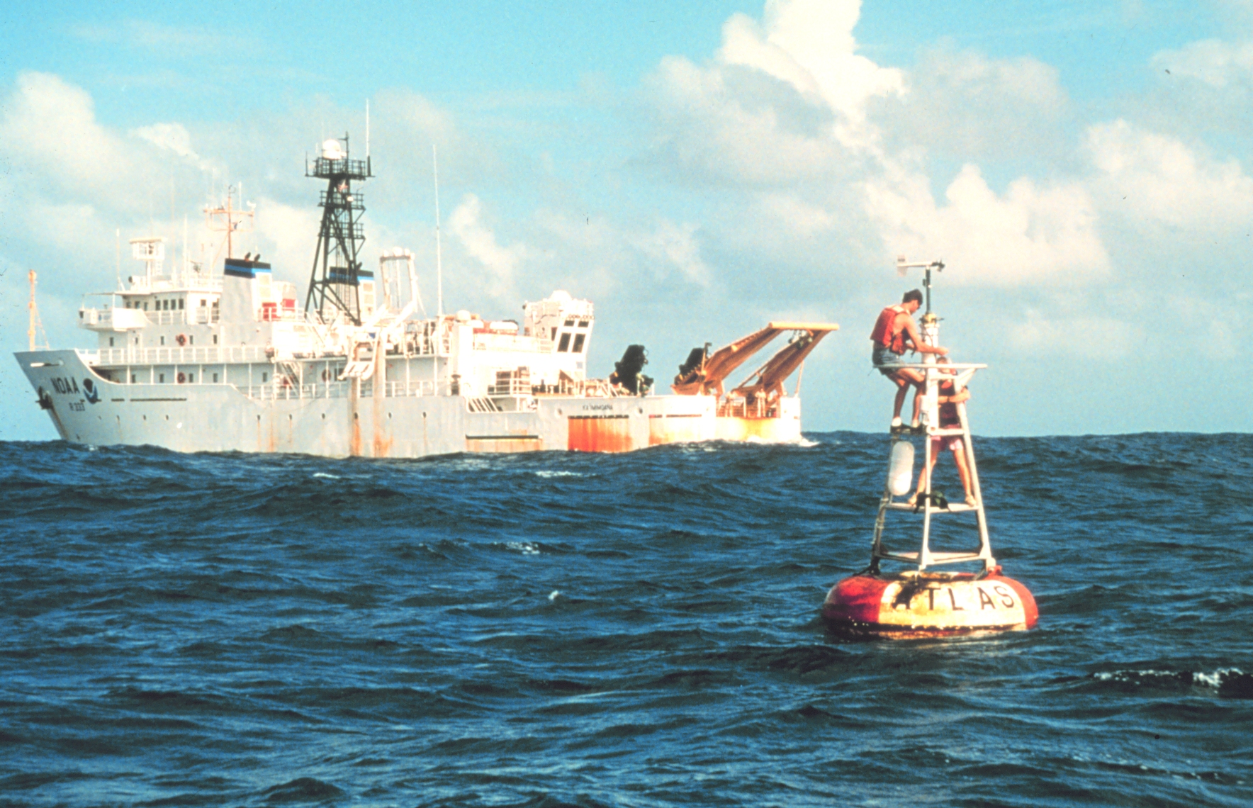
At about four o’clock on a clear morning in the equatorial Pacific, a few hundred kilometres south of the Equator and a thousand kilometres west of nowhere in particular, the deck of the NOAAS Ka’imimoana – a 224-foot former U.S. Navy ocean-surveillance vessel that the National Oceanic and Atmospheric Administration had commissioned at Pearl Harbor on 25 April 1996 specifically to maintain a network of moored buoys – is lit by deck lamps and full of people in life jackets. The mooring on the aft deck is in two pieces. The first is a yellow fibreglass-over-foam toroid – a doughnut, 2.3 metres across, 660 kilograms in air, with a small aluminium tower carrying a propeller anemometer, an aspirated air-temperature-and-humidity probe, an Eppley pyranometer, a Paroscientific barometer, and a self-siphoning rain gauge. The second is a railroad-wheel scrap anchor, weighing close to two tonnes, which the engineer has bought from a U.S. scrap yard for about a hundred dollars. Between them will go 5 500 metres of mooring line: stainless-steel wire rope above, 8-strand nylon below. The wire-rope upper section will carry, clamped to it, ten thermistors at standard depths and a few salinity recorders. Cable fairings – thirty-five-centimetre airfoils, the engineer Hugh Milburn’s idea – will reduce drag from the Equatorial Undercurrent flowing eastward at a metre per second a hundred metres below.
By the time the sun is up the mooring is over the side. The anchor hits the seafloor 5 200 metres below. The toroid floats. Within an hour the Argos satellite radio inside the electronics cylinder has woken up, listened for a polar-orbiting satellite passing overhead at 850 kilometres altitude, and shouted, in 256 bytes, three numbers and a checksum: surface wind, sea-surface temperature, the temperature of the upper ocean at twenty metres’ depth. By the end of the watch, when the Ka’imimoana has steamed thirty miles to the next mooring site, the data is in CLS Toulouse and on its way to PMEL Seattle, to the Global Telecommunications System, to ECMWF Reading, to NCEP Camp Springs. Latency: six hours. The next forecast cycle will use it. The ship makes thirty more deployments and recoveries on the cruise. Each mooring it leaves behind transmits hourly for the year before the next ship returns to recover it.
This is what the equatorial Pacific looked like in late 1996. There were sixty-nine of these moorings deployed from 8 degrees north to 8 degrees south, on seven longitude lines from 165 degrees east (west of Papua New Guinea) to 95 degrees west (off Peru) – one third of the circumference of the Earth. They had cost the United States, France, Japan, and a coalition of partner states approximately thirty-five to forty million dollars over a decade to build out. They had been finished, as a basin-scale network, on the schedule that one PMEL physical oceanographer named Stanley Phillip Hayes had laid out on a sheet of paper at an international meeting in March 1987. Hayes had died at his home in Seattle, of leukaemia, on 14 July 1992, age forty-eight, with the network about two-thirds complete. His deputy Mike McPhaden had taken the directorship of the project office in August 1992 and finished the deployment in December 1994.
This is the story of those sixty-nine buoys. It is also the story of how the conceptual ENSO of Jacob Bjerknes, the operational forecast on a basement VAX of Mark Cane and Stephen Zebiak, and the predictability framework of Jagadish Shukla became, between 1985 and 1998, an actual functioning operational seasonal-forecasting system serving every major weather centre on Earth.
Where the previous posts left off
Our previous post ended at George Mason University in Virginia in the late 2010s, with Jagadish Shukla’s COLA running on commodity Linux clusters. The architectural through-line of that post was the predictability framework: monthly mean atmospheric states are predictable beyond Lorenz’s two-week deterministic chaos limit because slowly-varying boundary conditions – sea-surface temperature, soil moisture, snow cover, the seasonal cycle – supply a forecasting signal that classical chaos does not erase. Shukla’s December 1981 paper in the Journal of the Atmospheric Sciences was the formal statement. The framework was beautiful. The implementing infrastructure was missing.
The infrastructure problem of seasonal forecasting was that the slowly-varying boundary conditions were almost entirely unobserved. Atmospheric variables had been observed since the 1940s by the radiosonde network and since the late 1970s by polar-orbiting satellites. SST could be retrieved from satellite infrared imagery, with caveats. But the principal seasonal-forecast signal – the warm pool, the equatorial cold tongue, the slow east-west sloshing of the Pacific upper ocean that constitutes the El Nino-Southern Oscillation – was, in the early 1980s, observed by perhaps a few hundred volunteer observing ships passing through the tropical Pacific each year, by some scattered island weather stations, and by satellite SST retrievals that struggled with cloud cover and stratospheric aerosols.
What the ECMWF seasonal-forecast model that took its first operational form in 1997 needed, what the NCEP coupled forecasting system that became the Climate Forecast System in 2004 needed, what the IRI’s monthly multi-model ENSO plume that emerged through the late 1990s needed, was a real-time three-dimensional view of the upper ocean across the equatorial Pacific. The Cane-Zebiak model on the Lamont VAX in 1986 had shown that the model existed. Shukla’s 1981 paper had shown that the predictability existed. What did not exist, until 1994, was the data. The buoys that follow are how the data got there.
1982-83: the surprise that triggered TOGA
In the boreal autumn of 1982 something began to happen in the equatorial Pacific that the operational community did not see coming. Sea-surface temperatures off the coast of Peru began rising in October. By December the equatorial Pacific between 160 east and the South American coast was three degrees Celsius above climatology. By March 1983 it was the strongest El Nino in a century: equatorial sea-level had risen by 30 centimetres in some places, the Walker circulation had collapsed and reorganised eastward, the trade winds had reversed, the South Pacific Convergence Zone had shifted eastward by thousands of kilometres, and rainfall patterns from northern Australia to South America to the Horn of Africa had been thoroughly rearranged.
The standard institutional account, given by Mike McPhaden, Antonio Busalacchi, and David Anderson in their 2010 retrospective in Oceanography, is unambiguous in its framing. “This El Nino, the strongest of the twentieth century up to that time, caught the world completely by surprise. It was not predicted because no El Nino forecast models existed. Even more startling was the fact that it was not even detected until nearly at its peak.”1
The specific failures of the 1982-83 detection process are why TOGA-TAO came to exist at all. There were three.
First, no operational coupled atmosphere-ocean forecast model existed. The Cane-Zebiak intermediate-complexity model that we covered in Post 27 was still three years away from its 26 June 1986 Nature paper. The full-physics coupled GCMs at GFDL and NCAR were not yet running with realistic ENSO behaviour. The seasonal-forecast capability of the operational meteorological community in 1982 was, in any practical sense, nil.
Second, the satellite-based sea-surface-temperature retrievals that were the principal real-time observation of tropical Pacific SST in 1982 were systematically biased cold by stratospheric aerosols from the El Chichon eruption. El Chichon, a volcano in the southern Mexican state of Chiapas, had erupted on 28 March and again on 4 April 1982. Its plume injected approximately seven megatonnes of sulphur dioxide into the stratosphere, where it formed a sulphate-aerosol veil that sat across the tropical Pacific for most of 1982. Satellite infrared sensors scattered the infrared signal in a way that made the rising SSTs look roughly normal. The most consequential satellite observing system the world had for tropical SST was, in mid-1982, blinded by a Mexican volcano.
Third, the canonical El Nino precursor patterns described in Eugene Rasmusson and Thomas Carpenter’s May 1982 Monthly Weather Review paper – the empirical baseline that NOAA’s Climate Analysis Center used to monitor for the onset of warm events – did not appear in 1982.2 The 1982 event began with a different evolutionary signature than the canonical Rasmusson-Carpenter El Nino. By the time the forecasters at CAC realised what was happening, the event was nearly half over.
The cost of the failure was substantial: approximately eight billion 1983 United States dollars in direct economic damages globally, between thirteen hundred and two thousand deaths worldwide, the further catastrophic collapse of the Peruvian anchoveta fishery, eleven-foot rainfall in northern Peru against a normal of six inches, drought across Australia and Indonesia, the Pacific Ocean’s first cyclones in living memory hitting Tahiti. The professional humiliation was extensive and bipartisan. The Rasmusson-Carpenter operational ENSO monitoring system at CAC had been declared in 1982 to be the world’s best ENSO diagnostic capability; it had failed to detect the largest event of the century until the event was nearly at its peak. The post-mortem in the World Climate Research Programme and the Intergovernmental Oceanographic Commission committee structure through 1983-1984 led directly to the formal creation of the Tropical Ocean Global Atmosphere programme as a ten-year international research effort with operational observing-system development as its central goal.
The institutional pre-history goes back further. In 1978 the IOC and the Scientific Committee on Ocean Research had jointly established the Committee for Climatic Changes and the Ocean (CCCO), under the chairmanship of Roger Revelle.3 One of CCCO’s charter members was the British-Australian theoretical oceanographer Adrian Edmund Gill (born 22 February 1937 in Melbourne, then at Cambridge), whose 1980 paper “Some simple solutions for heat-induced tropical circulation” in QJRMS had given the climate-dynamics community the analytical framework for the atmospheric response to a tropical SST anomaly. Gill’s atmosphere – a steady-state shallow-water response on a beta plane to a heating function – was the atmospheric component the Cane-Zebiak coupled model would use four years later. Gill became the first chairman of the TOGA Scientific Steering Group at TOGA’s 1985 launch. He did not see the array deployed: Gill died of cancer at Cambridge on 19 April 1986, age forty-nine, two months before the Cane-Zebiak Nature paper appeared.4 His Scientific Steering Group chairmanship passed to George Philander of Princeton.
The TOGA programme was launched in January 1985 under the World Climate Research Programme, co-sponsored by the IOC of UNESCO, the WMO, and the International Council of Science. It ran for ten years, through December 1994. Its three formal goals, as McPhaden’s retrospective sets them out, were “to determine the predictability of the coupled ocean-atmosphere system in the tropics on seasonal-to-interannual time scales, to understand the mechanisms responsible for that predictability, and to establish an observing system to support climate prediction.”1 That third goal was the one that became, on the American side and along the equatorial Pacific specifically, the moored-buoy array.
Stan Hayes (1944–1992)
There is no widely-available free-licensed photograph of Stanley Phillip Hayes. He was one of the senior physical oceanographers at NOAA’s Pacific Marine Environmental Laboratory at Sand Point on the western shore of Lake Washington in Seattle through the 1980s; he had built his career there from approximately 1980 onwards; he was awarded NOAA’s Department of Commerce Gold Medal in 1989; he died at age forty-eight in Seattle, of leukaemia, in mid-July 1992. He left behind a deployment plan for a basin-scale tropical-Pacific moored-buoy array that he had drawn up in 1987 and a programme office at PMEL that was about two-thirds of the way through executing it. The standard biographical reference is Mike McPhaden’s December 1996 eulogy in the Journal of Climate, “Stanley P. Hayes, 1944-1992.”5
The McPhaden eulogy gives the dates as 1944-1992 without further detail of birth date or place. The PMEL institutional pages name him once in the body text of the “Building TAO” history. The English Wikipedia has no article on him. The pattern is the same one we encountered with Aksel Wiin-Nielsen in the ECMWF post, with Daniel Slotnick in the ILLIAC IV post, and with William Bourke in the same ECMWF context: a senior figure in operational atmospheric or oceanographic computing whose career sits in the institutional shadow of larger and more public scientific figures, and whose photograph nobody has thought to release into the commons. The TAO array is, in this sense, the more durable monument.
From the late 1970s onwards, PMEL had been operating moorings on the equator at 110 degrees west under NOAA’s Equatorial Pacific Ocean Climate Studies (EPOCS) programme. The moorings were oceanographic moorings of the standard 1970s pattern: heavy current-meter moorings with Savonius rotors, vector-averaging vane indicators, and magnetic-tape data loggers that one read six months later after the mooring was recovered. They were what Walter Munk and Henry Stommel and the founding generation of physical oceanographers had taught their students to build. They were also, by the late 1970s, fundamentally incompatible with the operational forecasting need that was about to come.
In 1980 Hayes’s group achieved the first real-time transmission of air temperature and sea-surface temperature from a current-meter mooring at 0 degrees, 110 degrees west, over the Argos satellite system. In October 1983 wind measurements were added. Between January 1983 and March 1984, Hayes and the PMEL Engineering Development Division – founded in the early 1970s by Hugh Milburn, and including the surface-mooring engineer P. D. McLain – designed and bench-tested a new low-cost surface buoy with a thermistor cable hanging beneath it. The design philosophy was that real-time basin-scale tropical Pacific monitoring would only work if the moorings were inexpensive enough to deploy in large numbers. They called it the Autonomous Temperature Line Acquisition System – ATLAS.
The first ATLAS prototype was deployed in April 1984 at 2 degrees north, 108 degrees west: subsurface temperature data telemetered in real time from a buoy in 5 000 metres of water. By October 1984 ATLAS moorings had been established at 2 degrees north and 2 degrees south along 110 west. By July 1985 the array had expanded into the western Pacific with TOGA funding and French support from ORSTOM (later renamed the Institut de Recherche pour le Developpement), at 2 degrees north and 2 degrees south on 165 east. The science was working. The hardware was working. The next question was the basin scale.
In March 1987, with ten ATLAS moorings then deployed, Hayes presented the formal Tropical Atmosphere Ocean (TAO) array concept at international meetings: a basin-spanning network of approximately seventy moorings on roughly seven longitude lines from the western Pacific warm pool to the South American coast, fully telemetered, fully real-time, fully operational. The Milburn and McLain technical paper had appeared at the IEEE/MTS Marine Data Systems International Symposium in New Orleans the previous April.6 The first formal description of the array as a scientific programme was Hayes, Mangum, Picaut, Sumi, and Takeuchi, “TOGA-TAO: A Moored Array for Real-time Measurements in the Tropical Pacific Ocean,” in the Bulletin of the American Meteorological Society in March 1991.7
The build-out chronology, from PMEL’s “Chronology of TAO” page, runs: June 1986, wind data integrated; July 1988, TAO data distributed via the GTS through Service Argos – the operational shift that made TAO data available to NCEP and ECMWF in real time; 1989, Department of Commerce Gold Medal “for his leadership in the EPOCS Program”; October 1989, TAO Project Office formally established at PMEL with Hayes as Director; November 1989, humidity sensors added; January 1990, Japan joined under JAMSTEC sponsorship; May 1990, first PROTEUS mooring with a downward-looking ADCP; August 1991, rain gauges and pyranometers; February 1992, Korea joined; June 1992, TAO data on the public internet via a pre-Web FTP service. Across 1985-1992 the array grew from two moorings on 110 west to about forty-five moorings across seven longitude lines.
In late 1991 or early 1992 – the date is not in the eulogy and is treated discreetly in the institutional memoir – Hayes was diagnosed with leukaemia. He continued to work through the winter and spring of 1992. McPhaden was, by this point, the senior PMEL oceanographer in Hayes’s group and the obvious deputy. He took over the day-to-day coordination of the project office during Hayes’s illness. The international partnerships continued; the deployment cadence continued; the data flow continued.
Hayes died on 14 July 1992, age forty-eight, in Seattle.5 McPhaden became Director of the TAO Project Office in August 1992. About forty-five of the planned seventy moorings were in the water on the day of Hayes’s death.
ATLAS, in detail
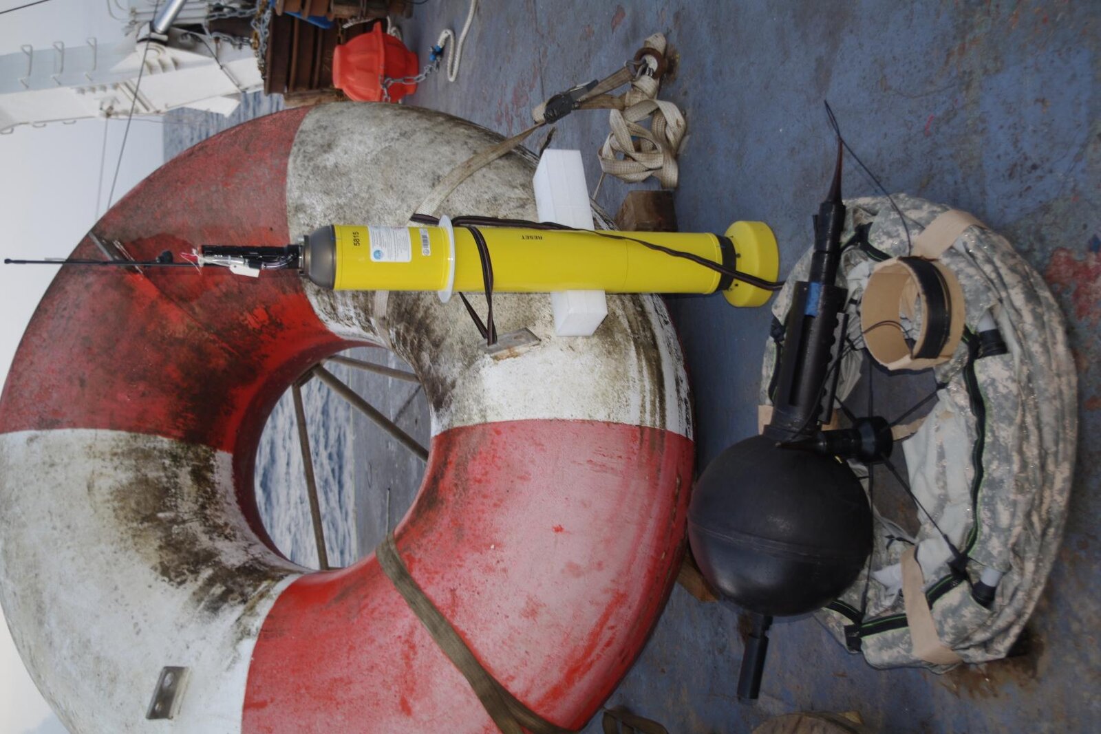
The ATLAS surface mooring is, by deep-sea oceanographic standards, almost embarrassingly modest. That is also the point.
The hull is a 2.3-metre fibreglass-over-foam toroid weighing approximately 660 kilograms in air, with net seawater buoyancy of about 2 300 kilograms. An aluminium tower bolted to the toroid carries the meteorological sensor suite: an R. M. Young propeller-vane wind sensor at 3.8 metres above the sea surface, a baffled-housing air-temperature thermistor, a Rotronic relative-humidity probe, a Paroscientific barometer, an Eppley pyranometer, and an R. M. Young rain gauge. The electronics tube – 1.5 metres long, 27 kilograms – sits in the well of the toroid: a custom-firmware data logger, a lithium primary battery pack, an Argos satellite radio at 401.65 megahertz, and the multiplexer board that addresses the subsurface sensors.
Below the toroid the mooring line goes down. The upper section, in the upper roughly 700 metres, is 9.5-millimetre stainless-steel wire rope, jacketed up to 12.7 millimetres for fish-bite protection. The thermistors – ten of them, in the eastern Pacific configuration at 20, 40, 60, 80, 100, 120, 140, 180, 300, and 500 metres; in the western Pacific shifted to 25, 50, 75, 100, 125, 150, 200, 250, 300, 500 metres to better resolve the deeper warm-pool thermocline – clamp to the wire. The lower section, from about 700 metres down to the anchor, is 19-millimetre 8-strand nylon. The anchor is railroad-wheel scrap, between 1 900 and 2 000 kilograms, bought from U.S. scrap yards. Most equatorial Pacific TAO sites sit in 4 000 to 5 500 metres of water.
The engineering insight that made the basin-scale array possible is one that is easy to overlook in retrospect because, by 2026, it is just how moored buoys work. At the equator the strong surface currents – the Equatorial Undercurrent at 100-150 metres depth flowing eastward at a metre per second, the South Equatorial Current that can reverse during El Nino – would normally drag a taut-line mooring far off station. Hugh Milburn’s solution was a series of 35-centimetre airfoil-like fairings, clamped to the wire-rope mooring line in the upper 200 metres. The fairings reduced drag and let a deep equatorial mooring stay on station. PMEL was granted United States Patent 7 244 155 for this design in 2007, two decades after the initial deployment. It was the first time anyone had reliably moored in waters greater than 4 000 metres on the Equator.
Cost per mooring per year, in late-1990s PMEL accounting: approximately 500 000 United States dollars, ship time and Argos fees included. The total United States TOGA-TAO programme cost across the 1985-1994 decade was approximately 35 to 40 million dollars. For comparison, a single Cray Y-MP at NCAR cost about 20 million dollars in 1990 and ran a single forecast. The TOGA-TAO array, for less than twice the cost of a Cray Y-MP, observed one-third of the circumference of the Earth in real time for a decade.
The array’s design lifetime was one year between recoveries – extended from the original six-month design goal as fish-bite-resistant cabling and more durable surface electronics were proven. The 1990 PROTEUS variant, with its downward-looking ADCP in the toroid base, ran in parallel through 1995, when fish-backscatter contamination of the acoustic-Doppler returns forced PMEL to abandon the design. PROTEUS hardware was incorporated into the NextGeneration ATLAS, first deployed operationally in May 1996, made the exclusive design in November 2001 – the original 1985-design ATLAS retired after seventeen years. NextGeneration ATLAS introduced inductively coupled subsurface sensors that addressed each thermistor individually on a bare-wire data path, and per-channel sample-rate flexibility down to one-minute intervals for rainfall. The standard meteorological suite expanded from three variables (wind, air temperature, SST) to seven, and subsurface salinity was added at selected depths.
The T-Flex mooring, first deployed in March 2011, replaced the entire 1990s electronics suite with a drop-in canister carrying an Iridium modem and an internal data-logging capability that recovered the full high-resolution record on recovery rather than only what had fit through the satellite link. T-Flex returned hourly data via Iridium in WMO BUFR format, bypassing Argos entirely. By the early 2020s most of the TAO array had migrated to T-Flex or to the NDBC-managed TAO Refresh successor. But the basic geometry – toroid, tower, wire rope, thermistors at standard depths, 9-tonne railroad-wheel anchor on the abyssal plain – has not changed since 1984.
The Argos satellite uplink
The piece of infrastructure that made the entire system possible is one that nobody outside the polar-orbiting-satellite community typically thinks about. It is also, in 2026, forty-eight years old.
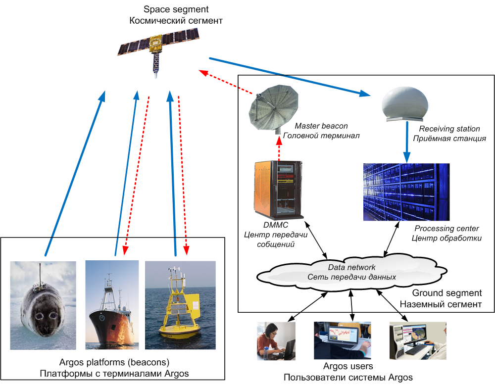
The Argos system is a polar-orbiting environmental data-collection-and-relay satellite system created in 1978 as a joint French-American effort, formalised through a 1974 Memorandum of Understanding among CNES (the French space agency), NASA, and NOAA. Architecturally it is the simplest possible thing: a one-way uplink from low-power surface transmitters to whichever polar-orbiting satellite happens to be passing overhead, with the satellite acting as a store-and-forward repeater to a small number of ground stations.
First service was in 1978, on the TIROS-N polar-orbiting satellite. By the early 2000s the constellation had grown to include the European MetOp series, the Indian-French SARAL satellite, and others. The polar orbits sit at approximately 850 kilometres altitude with a roughly 100-minute period; an Argos-equipped satellite passes over any given equatorial point several times a day. The transmitter sends a short data burst – 3 to 31 bytes per message – at intervals of 60 to 200 seconds. The satellite, when overhead, decodes the burst, time-stamps it, computes the transmitter location by Doppler shift, and re-transmits the data to ground stations at Wallops Island, Virginia, and Lannion, Brittany. Service Argos – the operational arm, since 1986 the CNES subsidiary CLS at Toulouse, with its US subsidiary in Lanham, Maryland – processes the data and inserts a real-time subset on the WMO Global Telecommunications System several times a day, where ECMWF, NCEP, JMA, the Australian Bureau of Meteorology, Meteo-France, and the rest of the operational forecast community ingest it. End-to-end latency in the late 1980s was typically 4 to 12 hours; by the mid-1990s it was typically 2 to 6 hours.
The fundamental shift that Argos enabled is a piece of operational practice that is now so completely the norm that it is hard to remember it was, in the early 1980s, a research curiosity. Walter Munk, Henry Stommel, Henry Bigelow, and the founding generation of physical oceanographers had been used to seeing their data months after collection: the ship recovered the mooring; the magnetic-tape logger went into the laboratory; the data was processed; the report was written; the result reached the journal in another year. A six-month round trip from observation to interpretation was the late-1970s norm. The post-Argos generation of TOGA-era oceanographers were used to seeing their data the same day. A six-month turnaround makes a mooring’s data useful for retrospective analysis but unusable for operational forecasting; a six-hour turnaround makes the same data usable for real-time ENSO monitoring and for forecast-model initialisation. The infrastructure that NCEP began running in the late 1980s, the operational seasonal-forecast systems at ECMWF that emerged from 1992 onwards, the modern subseasonal-to-seasonal forecast products produced daily by every major weather centre in 2026 – all of them depend on this Argos-enabled real-time data flow.
Argos was a fundamentally cooperative arrangement between France and the United States. The 1974 CNES-NASA-NOAA Memorandum of Understanding is, in retrospect, one of the more consequential pieces of low-bandwidth telecommunications infrastructure of the late twentieth century. The migration to Iridium from around 2010 increased available bandwidth by orders of magnitude and let the T-Flex moorings transmit hourly all-channel data instead of daily means. But the basic operational pattern – transmit, store-and-forward, GTS injection, hours of latency – is the Argos pattern.
NOAAS Ka’imimoana
A buoy array is only as strong as its servicing schedule. From the 1984 prototype through the mid-1990s, PMEL deployed and recovered ATLAS moorings opportunistically from chartered NOAA, Scripps, and Woods Hole research vessels. The lack of dedicated ship time limited how aggressively the array could grow. NOAA’s answer was a ship.
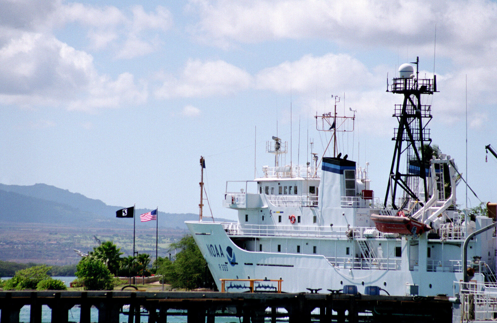
The vessel that became NOAAS Ka’imimoana – Hawaiian for “ocean seeker” – had been built in 1989 as USNS Titan (T-AGOS-15), a U.S. Navy ocean-surveillance vessel. She was transferred from the Navy to NOAA on 31 August 1993, the day she was retired from Navy service, and commissioned in NOAA service as NOAAS Ka’imimoana (R 333) on 25 April 1996 at Pearl Harbor. She was 224 feet long, 1 650 tons light displacement, with berths for 33 (including up to 12 scientists), 950 square feet of lab space, three cranes, a J-frame and an A-frame on the stern, a brailing winch and a CTD winch, and a 22-foot rigid-hulled inflatable for buoy-rider work alongside deployed moorings. She was the only ship in the NOAA fleet dedicated solely to climate research.
From 1996 to 2012 she ran four to six TAO-servicing cruises per year, each visiting fifteen to twenty mooring sites. During each cruise she also collected CTD profiles, underway ADCP, thermosalinograph and surface-meteorological data, deployed Argo profiling floats and surface drifters, and transmitted incoming TAO mooring data to PMEL Seattle in real time. The combined effort – a dedicated ship, a steady deployment-and-recovery cadence, a small specialist crew of NOAA Corps officers and PMEL technicians – kept data return above 80 per cent through the late 1990s and 2000s.
In 2012, facing budget pressure, NOAA effectively withdrew her from active TAO duty. She was formally decommissioned on 18 June 2014. The successor for tropical-buoy work was NOAAS Ronald H. Brown, commissioned 19 July 1997, which began running TAO-servicing legs alongside her primary scientific missions. The decommissioning of Ka’imimoana in 2012-2014 was, in retrospect, an operational signal that NOAA’s institutional commitment to sustained TAO operations was weakening. The data-return collapse to 28 per cent in March 2014 traces directly to her absence. For most of the post’s central decade, however, Ka’imimoana was the workhorse: 200 days a year at sea, four hundred mooring deployments and recoveries across her service life. Many of the still photographs of TAO ATLAS moorings on Wikimedia Commons in 2026 – including the one at the top of this post – are Ka’imimoana photographs.
Mike McPhaden completes the array
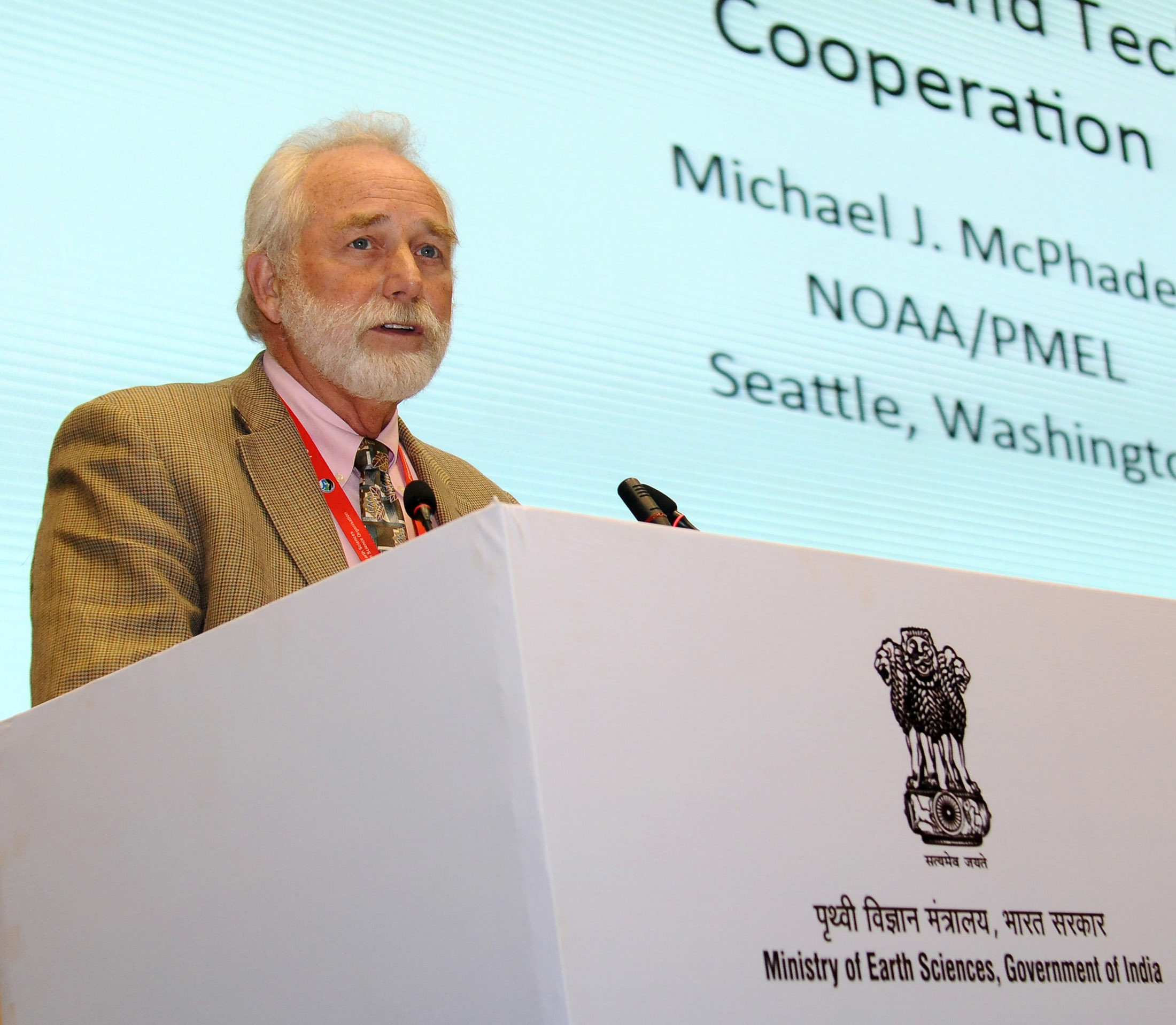
Michael James McPhaden was born in 1953. He took his B.S. in Physics at the State University of New York at Buffalo in 1973, magna cum laude. His Ph.D. in Physical Oceanography was from the Scripps Institution of Oceanography at UC San Diego in 1980; the dissertation title was “Models of the Equatorial Ocean Circulation.” From 1980 to 1982 he was a Research Scientist at NCAR in Boulder; from 1982 to 1984 a Visiting Research Scientist at the Joint Institute for the Study of the Atmosphere and Ocean at the University of Washington in Seattle; from 1984 to 1986 a Research Assistant Professor at the University of Washington; and from 1986 onwards an Oceanographer at PMEL, rising through the senior-research-scientist ranks. He had been Hayes’s deputy on the TAO programme for several years before he took the Project Office directorship in August 1992 in the immediate aftermath of Hayes’s death.
His job from August 1992 through December 1994 was, in some sense, simple. Hayes had set out the design, proven the technology, established the international partnerships, and got the funding through 1992. The remaining twenty-some moorings needed to go in the water on schedule. The data products needed to be validated at scale. The operational infrastructure to support 24/7 real-time data flow to NCEP and ECMWF and other major weather centres needed to be built. The institutional pattern for sustained operations beyond TOGA’s formal end-date of 31 December 1994 needed to be established. He did all four.
The array was completed in December 1994 on the schedule that Hayes had laid out in 1987. The final count was 64 ATLAS moorings plus 5 deep-ocean current-meter moorings: a total of 69, close to but not exactly the originally targeted seventy.8 The array spanned 8 degrees north to 8 degrees south in latitude, and 137 degrees east (west of Papua New Guinea) to 95 degrees west (off Peru) in longitude. There were approximately seven longitude lines, with finer resolution near the equator. The cooperating Japanese TRITON moorings, deployed by JAMSTEC in the western Pacific, would join the system in January 2000, at which point the combined network was renamed TAO/TRITON. The fifteen-author McPhaden et al. paper “The Tropical Ocean-Global Atmosphere observing system: A decade of progress,” published in the Journal of Geophysical Research in 1998, is the canonical decade-summary paper.9 It was written four years after Hayes’s death; McPhaden is first author.
What the array had become, by December 1994, was the first global-scale, real-time ocean-atmosphere observation system in history. There had been, before TOGA-TAO, oceanographic arrays of comparable physical size: the IGY of 1957-58, the FGGE special-observing periods of 1979, the various ship-of-opportunity XBT lines. None of them had been real-time. None of them had run continuously for years. None of them had been integrated into the operational forecasting workflow of every major weather centre. TAO was. By July 1988, when Service Argos had begun injecting the data on the GTS, the array was an operational source for NCEP, ECMWF, and any other centre that took the WMO standard data feed. By June 1992, with the data on the public internet via PMEL’s FTP service, any climate scientist anywhere could pull the latest mooring report. The thing the operational seasonal-forecast pipeline of Posts 27, 34, and 35 had needed – but did not have – in the early 1990s, it now had.
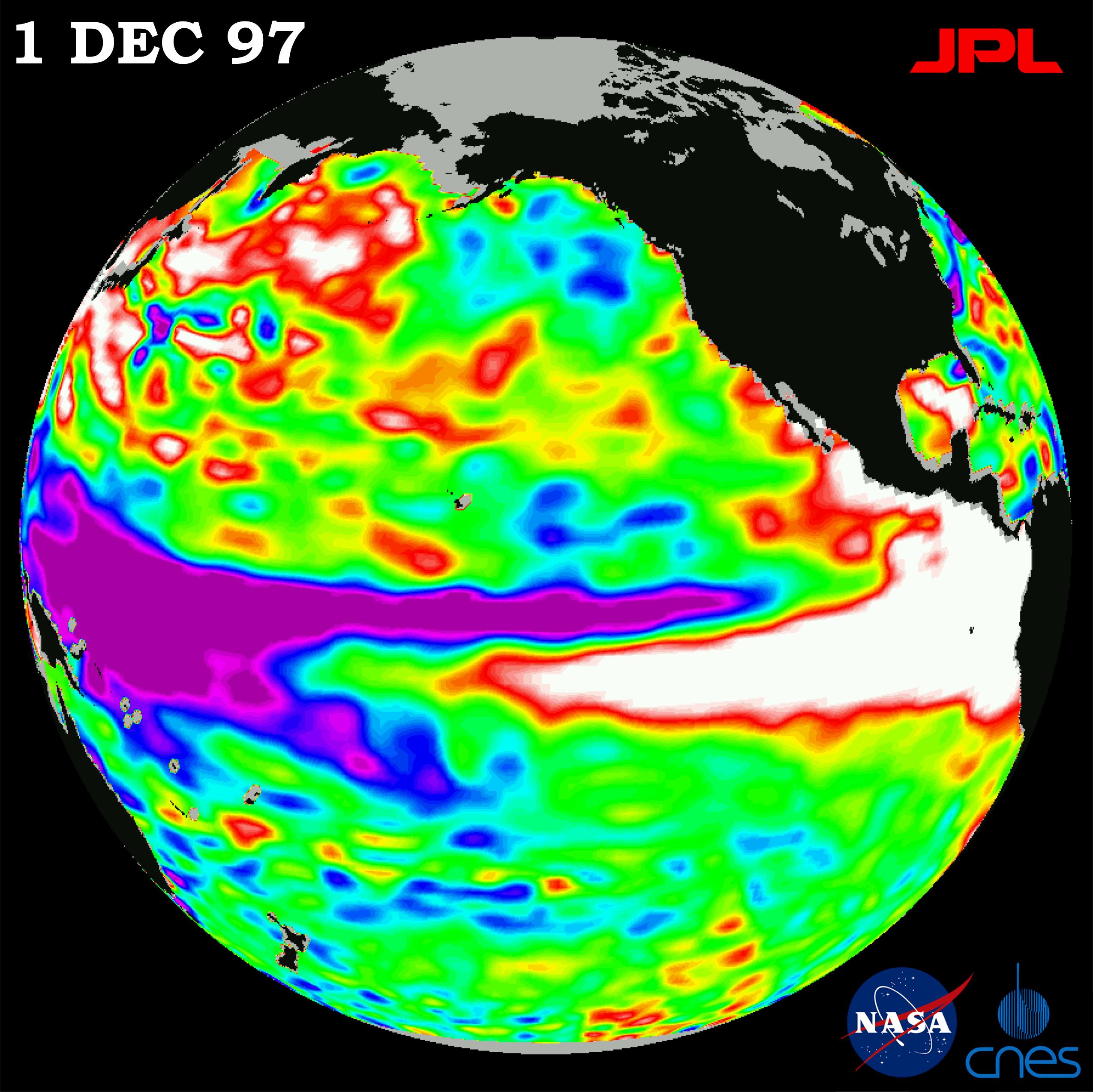
1996-1997: the array sees a warm wave coming
In the boreal autumn of 1996 a slow accumulation of warm water in the western equatorial Pacific began to register on the array. This was the standard precursor to a major El Nino event: a deeper-than-normal thermocline, sea-surface temperatures about half a degree Celsius above normal in the western basin. The basin must be charged with warm water in the west before the discharge phase that becomes El Nino. The TAO subsurface thermistors were, in this period, the principal observation: satellite SST retrievals could see the surface but not the warm reservoir building up below the western Pacific thermocline. The array could.
Through late 1996 and early 1997 a series of westerly wind bursts appeared on the moorings of the western Pacific warm pool, associated with the Madden-Julian Oscillation – the principal mode of equatorial atmospheric variability on the 30-90-day timescale. The wind bursts registered on the moorings as eastward displacement of the Walker rising branch, westerly wind anomalies on the equator lasting several weeks, and – crucially – subsurface warm anomalies propagating eastward at Kelvin-wave speed, approximately 2.7 metres per second on the equatorial waveguide, reaching the eastern Pacific in two months. By January 1997 TAO subsurface thermistors in the central Pacific were detecting unusually warm subsurface water; by April surface anomalies were “fully established”; by May they exceeded 5 degrees Celsius off South America; by September the equatorial Pacific between South America and the dateline averaged 2 to 4 degrees Celsius above normal. McPhaden’s Science paper “Genesis and evolution of the 1997-98 El Nino” identifies the genesis of the event with the second of the wind bursts in March-April 1997, although the precursor warming was visible in TAO subsurface data months earlier.10
The forecasts that the operational community made on this evolving situation were a mixed performance. The within-1997 contrast among the various models is instructive.
The Cane-Zebiak coupled model – the model whose 1986 Nature paper had started the operational ENSO-forecasting era and which we covered in Post 27 – was issuing experimental long-lead forecasts in the NCEP/CPC Experimental Long-Lead Forecast Bulletin under the personal supervision of Mark Cane and Stephen Zebiak.11 Performance during 1996-97 was mixed. The model’s January 1997 forecast called for “continuation of somewhat below normal Nino 3 conditions, with strongest negative anomalies for winter 1996-97” – weak La Nina conditions, exactly the opposite of what was about to happen. By March-April 1997 the model had reversed and was correctly predicting strong El Nino conditions for the second half of 1997, but only after the warming was already under way and being assimilated into the model’s ocean state. Across the suite of models surveyed in Anthony Barnston, Michael Glantz, and Yuxiang He’s 1999 BAMS postmortem, Cane-Zebiak underpredicted the 1997-98 event at every long-lead horizon prior to mid-1997.12 Cane himself, in a 2018 National Science Review interview, has been candid: “The model said no – and then it would happen a year later.”13
The European Centre for Medium-Range Weather Forecasts had been developing its own coupled seasonal-forecast system through the early 1990s under T. N. Stockdale and D. L. T. Anderson in the Operational Department at Reading. The ECMWF system was the only operational system that successfully predicted, two seasons in advance, the rapid rise of SST anomalies in May 1997. Stockdale, Anderson, Alves, and Balmaseda’s 1998 Nature paper reported that the system, run on data through January 1997, had predicted a +2 degrees Celsius Nino 3.4 anomaly for the December-January-February 1997-98 season; verification was +2.4 degrees Celsius, lead time approximately eleven months.14 The prediction was experimental, was not publicly released before it verified, and did not influence the operational forecast community in real time. ECMWF’s first formal operational seasonal-forecast system, System 1, was not introduced until 1997. The Stockdale et al. paper appeared in Nature in March 1998, after the event had peaked.
The forecast that did drive the operational and public-affairs response was issued by NOAA’s National Centers for Environmental Prediction Climate Prediction Center. The NCEP Climate Forecast System (CFS) – NCEP’s operational coupled atmosphere-ocean model – was, in 1997, still under development under the leadership of Ants Leetmaa, founding Director of the Climate Prediction Center, and Ming Ji of NCEP’s Environmental Modeling Center. CFS would not become fully operational until August 2004 (CFSv1) and March 2011 (CFSv2). What was operational at NCEP in 1997 was a development version of that system, plus statistical and statistical-dynamical ENSO monitoring tools, plus the weekly ENSO Diagnostic Discussions. By 1997 the predecessor system was a forecast-quality coupled GCM running monthly with TAO and Reynolds optimal-interpolation SST initialisation.
The crucial NCEP forecast was issued on 26 June 1997.12 It was the official CPC “Climate Outlook” and “ENSO Diagnostic Discussion” for the upcoming North American winter. It predicted, with explicit reference to the developing El Nino: above-normal precipitation across California, the southwestern US, the southern Gulf states, and the southeastern US; below-normal precipitation across the Pacific Northwest; above-normal temperatures across the northern half of the country; and wetter and stormier conditions across the southern third. Every one of these was qualitatively correct. The Barnston, Leetmaa, Kousky et al. 1999 BAMS postmortem called it: “Heavy winter precipitation across California and the southern plains-Gulf coast region was accurately forecast with at least six months of lead time, and dryness was also correctly forecast in Montana and in the southwestern Ohio Valley. The warmth across the northern half of the country was correctly forecast, but extended farther south and east than predicted.”12 This was the single most successful operational long-lead seasonal forecast in the history of the National Weather Service up to that time.
The forecast was, in a fundamental sense, based on the TAO array. The June 1997 forecast was issued at the moment when the array’s subsurface thermistors were showing – in real time, on the GTS, available to forecasters at NCEP and to the public at PMEL’s website – a strongly developing warm subsurface anomaly across the central and eastern equatorial Pacific. The data was already telling the operational meteorologists what the answer was going to be. The forecast that the meteorologists wrote was the consequence.
The 1997-98 El Nino
Through the boreal summer of 1997 the event grew with extraordinary speed. Each westerly wind burst excited a new downwelling Kelvin wave; each Kelvin wave, on reaching the eastern Pacific, pushed the thermocline deeper; the deepening thermocline reduced upwelling-driven cooling; the warming SST further weakened the trade winds; the weakened trades produced more eastward-shifted convection and more wind bursts. The Bjerknes feedback was running with particular vigour. McPhaden, summarising in his 1999 Science paper: “The El Nino developed so rapidly that each month from June to December 1997 a new monthly record high was set for SST.”10
By August 1997 the equatorial Nino 3.4 SST anomaly (the standard index, defined over 5 degrees north to 5 degrees south, 170 west to 120 west) exceeded +2 degrees Celsius. The thermocline depth in the eastern Pacific had been depressed by more than 90 metres relative to normal. The 28 degrees Celsius isotherm that normally marks the western Pacific warm pool now extended across the entire equatorial basin. The mature phase was attained in November-December 1997. Nino 3.4 SST anomaly peaked at approximately +2.5 degrees Celsius in November 1997. The Nino 1+2 region (off Peru and Ecuador) was even more anomalous: anomalies exceeding 5 degrees Celsius persisted from July 1997 through May 1998, with peak coastal anomalies of approximately 11 degrees Celsius above climatology reported off Peru in January 1998. Sea-level along the equator rose up to 34 centimetres above climatology in November 1997.
David Enfield’s 1999 paper in Bulletin of Marine Science gives the canonical comparison with 1982-83: “The 1982-83 and 1997-98 events, coming only 15 years apart, are generally comparable in magnitude and impacts, and are by far the strongest warmings observed since 1950.”15 In the eastern Pacific, 1997-98 was somewhat stronger and lasted longer; on most central-Pacific atmospheric indices, 1982-83 was at least equally strong. Klaus Wolter and Michael Timlin’s 1998 Weather paper concluded slightly in favour of 1982-83 as the stronger event overall using their objective Multivariate ENSO Index; Mike Davey and David Anderson, looking at SST, wind stress, sea-level pressure, and thermocline-depth indices, called the comparison “essentially a tie.”1617
What the 1997-98 event was, that the 1982-83 event had not been, was observed. The McPhaden 1999 Science abstract is the closest thing to a definitive technical statement of the contrast:
“The 1997-98 El Nino-Southern Oscillation was, by some measures, the strongest on record, with major climatic impacts felt around the world. A newly completed tropical Pacific atmosphere-ocean observing system documented this El Nino from its rapid onset to its sudden demise in greater detail than was ever before possible. The unprecedented measurements challenge existing theories for El Nino-related climate swings and suggest why climate forecast models underpredicted the strength of the El Nino prior to its onset.”10
The paired institutional statement is the Wallace, Rasmusson, Mitchell, Kousky, Sarachik, and von Storch 1998 paper in the Journal of Geophysical Research, which characterised the TOGA decade’s observational achievement.18
The collapse of the event was as dramatic as the onset. Between May and June 1998, the central and eastern equatorial Pacific cooled by 5 to 8 degrees Celsius in a matter of weeks. McPhaden’s Science paper records the most extreme observation: “At one location (0 degrees, 125 degrees W), SST dropped 8 degrees C in 30 days, more than 10 times the normal cooling rate.” The decay was driven by wind-forced upwelling Kelvin waves and reflected Rossby waves off the western boundary; the recharge phase of Fei-Fei Jin’s 1997 recharge-oscillator description was already under way, with a cool subsurface anomaly accumulating that would, by July 1998, become the strong La Nina event of 1998-2000.
The event was, by any reasonable definition, the best-observed El Nino in history. It was also the validation of the entire TOGA-TAO programme.
El Nino as household term
The 1997-98 El Nino was the moment “El Nino” entered American popular culture as a household phrase. The term had been used in scientific literature since the late nineteenth century, in the climate-science community since Bjerknes’s 1969 synthesis. It had got into mainstream press during 1982-83 but mostly as a foreign-news phenomenon. By autumn 1997 it was on the front page of every major American newspaper, the lead item on network news, and the punchline of the late-night monologues. Sarah Hare’s 1998 Eos note “Recent El Nino brought downpour of media coverage” counted the volume.19 Between June 1997 and June 1998 more than a thousand stories on El Nino appeared in The New York Times alone; the Washington Post, Los Angeles Times, and USA Today together contributed several thousand more.
The most famous individual instance is Chris Farley’s appearance on Saturday Night Live on 25 October 1997 – season 23, episode 4. Farley was the host, returning for what would be his last SNL hosting appearance before his death from drug overdose two months later on 18 December 1997. The skit, “Weather Scope,” cast him as a wrestling-style character named “El Nino” issuing pseudo-Spanish challenges to other personified weather phenomena. The bit ran for several minutes. The transcript exists at SNL Transcripts Tonight; the YouTube clip remains, in 2026, one of the most-viewed comedy moments of the 1997-98 American television season.20 The pop-culture moment was broader than a single SNL bit: by autumn 1997 there were T-shirts, novelty mugs, stickers, weather-merchandise products. Surf shops in California did brisk business in El Nino-themed surfwear. The Tonight Show and Late Show ran the term as a recurring punchline. The late-night comedy treatment was a marker of the term’s having graduated, in less than a year, from technical jargon to public idiom.
The Clinton administration treated the developing event as a serious operational challenge. Vice President Al Gore took the public-communications portfolio for the federal climate response. FEMA Director James Lee Witt, whom Clinton had elevated to cabinet rank in 1996 (the first FEMA director with that status), was the lead operational figure. NOAA Administrator D. James Baker Jr. was the lead public scientific spokesman. Vernon Kousky of CPC was the public face of CPC’s ENSO operations and the figure most often quoted in contemporary press. The campaign included NOAA press briefings from June 1997 onwards; the White House Climate Conference on 6 October 1997, attended by 100 broadcast meteorologists and most of the cabinet, covering both climate change and El Nino preparedness;21 President Clinton’s 22 October 1997 climate-policy speech at the National Geographic Society ahead of the December Kyoto negotiations; a presidential visit to California in February 1998; and the Project Impact disaster-preparedness initiative.
Vice President Gore, at the 26 February 1998 Project Impact press event: “Federal officials had the foresight to plan for the worst and prepare for the terrible impact of El Nino.”22 The framing was, on the substance, broadly correct. The forecasts had been used. Federal agencies pre-positioned resources, state governments prepared, agricultural extension services warned farmers, water managers adjusted reservoir operations, and individual households took precautions. The early warning had been operationally useful at every level of the response.
The 1997-98 impacts: what 23 000 deaths and $32-96 billion in damages bought
The 1997-98 El Nino, even with months of advance notice, was catastrophic. Damage estimates vary widely; figures most commonly cited in the post-event reviews are between US$32 billion (Sponberg 1999) and US$96 billion (Swiss Re 1999), with a central estimate near US$36 billion (Kerr 1999 in Science).23 The death toll most commonly cited is approximately 23 000 globally, with very wide uncertainty bounds; the UNEP-NCAR-UNU-WMO-ISDR assessment by Michael Glantz et al., “Lessons Learned from the 1997-98 El Nino: Once Burned, Twice Shy?” (October 2000), gives “more than 22 000 lives lost.”24 A 2023 re-analysis by Christopher Callahan and Justin Mankin in Science puts the five-year cumulative global economic loss attributable to the event, including secondary climate-modulated impacts, at approximately US$5.7 trillion.
The regional pattern was the canonical El Nino pattern, made unusually severe by the magnitude of the event. California recorded its wettest February on record (since 1895), with cumulative damages over US$550 million in the San Francisco Bay region alone. The Pacific Northwest, counter-intuitively, was predicted to be dry, because in strong El Nino years the storm track shifts south; the CPC forecast got this right. The southeastern United States experienced its wettest December-February on record (Florida 19.28 inches against a pre-1998 record of 15.14 inches; South Carolina 19.54 inches). Florida had the worst tornado outbreak in state history during a single 24-hour period in February 1998: 42 deaths. The Northeast set warmth records in Connecticut, Iowa, Michigan, Minnesota, New Hampshire, and Wisconsin; the 5-9 January 1998 ice storm killed 56 people and caused over US$2 billion in damages in Canada and over US$300 million in the United States.
Peru suffered catastrophic flooding, predicted by every forecast system: over 200 deaths, US$1.4 billion in damages, hundreds of thousands displaced; the anchoveta fishery collapsed and fishmeal-and-oil production fell by more than 80 per cent. Indonesia suffered the worst drought in fifty years. Approximately five to ten million hectares of forest burned across Sumatra and Kalimantan during 1997-98 – an area on the order of Hungary or South Korea. Smoke spread over eight Southeast Asian countries and affected an estimated 75 million people. According to Susan Page and colleagues’ 2002 Nature paper, the carbon released from burning peat was on the order of an entire year’s fossil-fuel emissions from Western Europe. Australia suffered drought, but less severely than 1982-83.
The pattern across eastern Africa was complicated. Kenya and Somalia had widespread flooding and a Rift Valley fever outbreak; WHO documented approximately 89 000 human cases of RVF and 200 to 250 deaths from the disease, plus a much larger flooding-related death toll. Tanzania reported 40 249 cholera cases and 2 231 deaths in 1997. Southern Africa drought was milder than predicted – a miss serious enough that Mark Cane himself, in a SciDev.Net interview, has cited Africa as a case where over-confident forecasts produced unintended economic harm: banks reportedly withdrew credit from farmers anticipating reduced incomes, and the actual drought was less severe than the forecasts had implied. Coral reefs, globally, suffered a mass-bleaching event; approximately 16 per cent of the world’s coral reefs died.
But the operational forecasts gave farmers, water managers, fishery operators, and emergency-management agencies months of advance notice. The Peruvian Ministry of Agriculture pre-positioned food stocks. Australian wheat production was hedged on commodity markets months in advance. The Illinois State Water Survey, in a contemporary analysis, estimated that the 1997-98 winter’s milder northern conditions across much of the United States had produced approximately US$19.6 billion in benefits, against US$4.2 to 4.5 billion in losses, for a net positive direct impact on the US economy. The institutional case for sustained operational seasonal forecasting was, after 1997-98, no longer in question.
What the 1997-98 forecast did to the institutions
The aftermath of the 1997-98 event reshaped the operational seasonal-forecast community in four specific institutional ways, each of which is the operational ancestor of a system in active use in 2026.
The Climate Prediction Center had been formally established in 1995 as one of the seven service centres of the newly-named National Centers for Environmental Prediction, succeeding the older Climate Analysis Center which had operated under the National Meteorological Center since the late 1970s.25 CPC’s founding mandate explicitly included operational seasonal forecasting; Ants Leetmaa was the founding director, in post until 1998. The 1997-98 event was CPC’s first major operational test, less than two years after its formal establishment. The Barnston et al. 1999 BAMS postmortem is, by the dry standards of operational meteorology, almost a celebration. The institutional case for sustained CPC operational seasonal forecasting was made by the post-event review.
The International Research Institute for Climate and Society (IRI) at Lamont-Doherty had been formally established in 1996 – one year before the 1997-98 event began – as a NOAA-Columbia partnership. The initiative went back to a 1992 NOAA-organised Climate Forecasts Forum at which a coalition of climate scientists (Mark Cane, Stephen Zebiak, Jagadish Shukla, V. Ramaswamy) and NOAA leadership (D. James Baker, Edward Frieman) had argued that the seasonal-forecasting capability emerging from TOGA needed an institutional home outside the national weather services. Walter Munk of Scripps was a senior advisor in the founding period, not a co-founder. Mark Cane was a founding scientific leader. Stephen Zebiak became IRI Director-General in 2003 and held the post until 2012. The IRI’s monthly multi-model ENSO forecast plume, which continues in 2026 as the canonical operational multi-model product, was issued for the first time during the 1997-98 lifecycle.
The NCEP Climate Forecast System (CFS) – the development version of which had run during the 1997-98 event – became fully operational as a coupled GCM in August 2004 (CFSv1; Saha et al. 2006), with CFSv2 following in March 2011. Both are direct descendants of the 1996-97 development system; both depend, for tropical-Pacific initialisation, on the TAO array. The ECMWF seasonal-forecast system evolved from the 1997 introduction of System 1 through System 2 (2002), System 3 (2006), System 4 (2011), and SEAS5 (November 2017) – the system in operation in 2026, a fully-coupled atmosphere-ocean ensemble seasonal-forecast system running on the same Cray and now Atos supercomputers we covered in Post 34. It depends, for its tropical-Pacific initialisation, on the TAO/TRITON array.
After 1997-98 the WMO formally adopted ENSO forecasting as a routine component of its operational mandate. The 1999 WMO retrospective on the 1997-98 El Nino and the subsequent Climate Information and Prediction Services (CLIPS) programme institutionalised ENSO forecasting as a service national meteorological services were expected to provide. The WMO Global Producing Centres framework that operates today – NCEP CFS, ECMWF SEAS5, UK Met Office GloSea, Meteo-France, Environment Canada, others – is the institutional descendant.
What the Cane-Zebiak forecast had been on the Lamont VAX in 1986 – a single experimental forecast from a single intermediate-complexity model in a single research group’s basement office – had become, by 2000, a routine operational service issued continuously by every major national weather centre on Earth. The TAO array was the observational substrate of the entire system.
PIRATA Atlantic 1997, RAMA Indian Ocean 2004
McPhaden’s career legacy was not only the Pacific.
In September 1997 – in the same month the 1997-98 El Nino was ramping up and CPC was issuing its first warnings – the Pilot Research Moored Array in the Tropical Atlantic (PIRATA) deployed its first two ATLAS moorings at 10 south 10 west and (in January 1998) at 8 north 38 west. The pilot paper appeared in BAMS in October 1998.26 PIRATA was a tripartite cooperation among the United States (NOAA/PMEL/AOML), France (IRD and Meteo-France), and Brazil (INPE and DHN). The principal architects were Mike McPhaden, Bernard Bourles of IRD, and Jacques Servain of IRD. The hardware was directly inherited from TAO: ATLAS moorings, the same satellite uplink, the same engineering office at PMEL Seattle. The motivation was scientific: the equatorial Atlantic exhibits its own coupled ocean-atmosphere variability – the meridional gradient mode and equatorial warm events – that affects rainfall in northeast Brazil, West Africa, and the Caribbean. The Atlantic is not the Pacific; the Bjerknes feedback is weaker, the basin narrower, the variability more spatially heterogeneous and lower amplitude. But the technology that worked in the Pacific worked in the Atlantic.
The deployment chronology was incremental: 10-mooring backbone by early 1999; ADCP at 0, 23 west in 2001; Brazilian “Southwest Extension” of 3 moorings in 2005; NOAA-AOML “Northwest Extension” of 4 moorings in 2006; a short-lived South-African-sponsored “Southeast Extension” 2006-2007; the configuration of 17 sites since 2007; CO2 sensors from 2008, turbulence-microstructure and dissolved-oxygen from 2014, a 20 south 10 west reopening in 2020. PIRATA’s operational difference from TAO is that no single nation has taken on the dedicated-ship role that Ka’imimoana played in the Pacific; servicing cruises rotate among French, Brazilian, and US vessels.
The third basin came later. The Research Moored Array for African-Asian-Australian Monsoon Analysis and Prediction (RAMA) was begun in 2004, building on pilot-scale arrays previously deployed by JAMSTEC and India’s National Institute of Oceanography. The defining paper is McPhaden, Meyers, Ando, Masumoto, Murty, Ravichandran, Syamsudin, Vialard, Yu, and Yu in BAMS April 2009.27 The original RAMA design called for 46 mooring sites between 15 north and 26 south. By 2009, 24 sites had been occupied. The expected completion year of 2012 slipped because of two unusual problems. The first was vandalism: tropical fishing fleets treated moored buoys as fish-aggregation devices, tangled their nets in the mooring line, and then cut the line to free their gear. McPhaden et al. 2010 documented bullet holes in buoy electronics tubes and sensors sawn off. PMEL responded with the “conehead buoy,” a smooth-walled hull with no boarding handholds. The second problem was piracy: the November 2009 ASCLME servicing cruise was curtailed by Somali pirate activity; it would have completed the 55 east line. RAMA’s national partnership is the most extensive in the global array, including NOAA, JAMSTEC, India’s Ministry of Earth Sciences, Indonesia, China’s State Oceanic Administration, France’s IRD, and the ASCLME programme covering nine Indian Ocean rim states. By the late 2010s RAMA was approximately two-thirds of the planned size; the most recent moorings were deployed in the Arabian Sea in 2019.
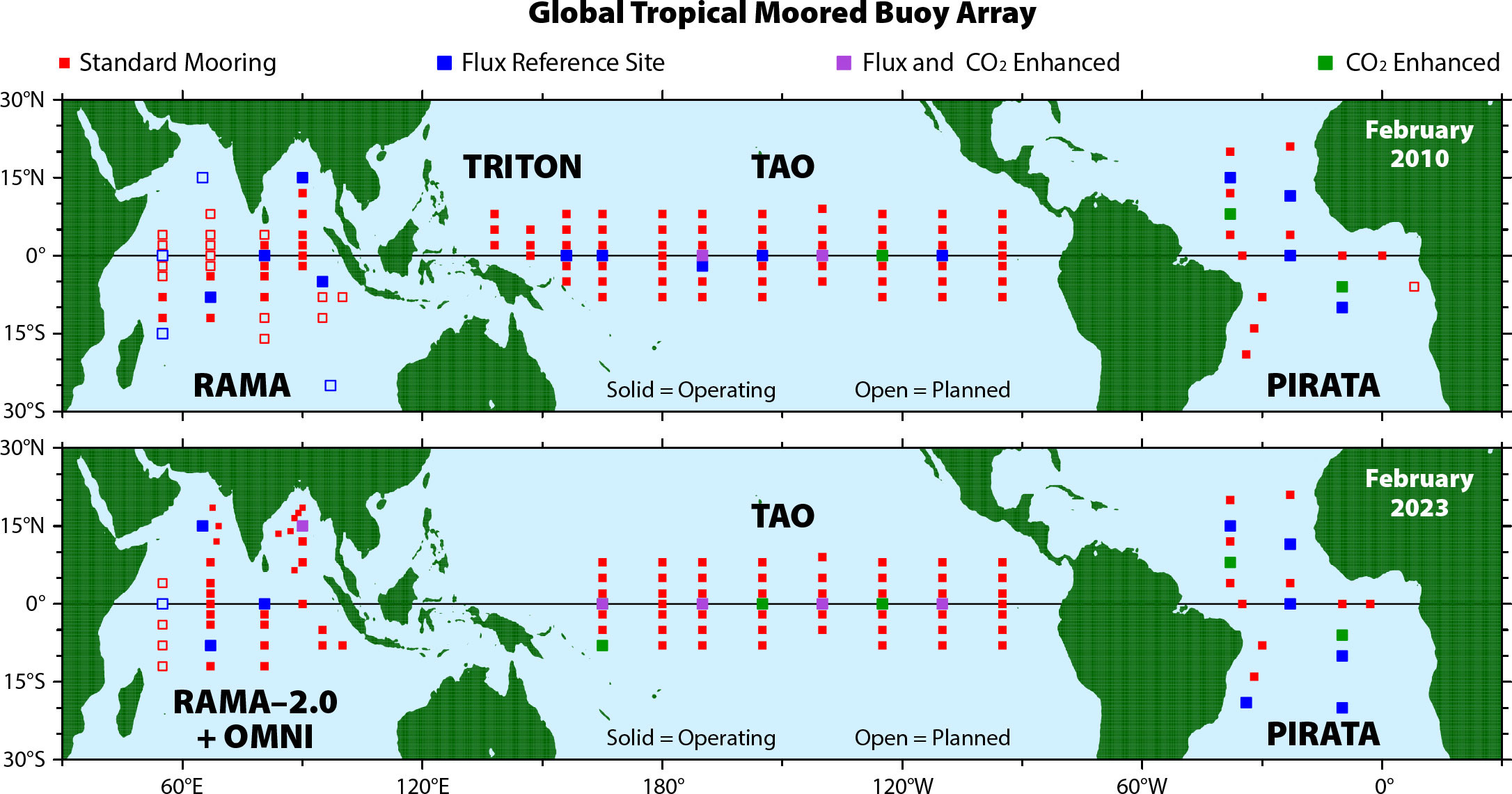
Together, TAO/TRITON in the Pacific, PIRATA in the Atlantic, and RAMA in the Indian Ocean form what McPhaden calls the Global Tropical Moored Buoy Array (GTMBA). The institutional structure – a multinational coalition organised through PMEL Seattle as the engineering hub, with operational ship time and scientific leadership distributed across a dozen countries – is, in 2026, McPhaden’s career legacy.
The 2012-2014 partial collapse
The TAO array’s institutional fragility became visible in the early 2010s. The transition from pure-research operations – under PMEL on TOGA-era programme funding – into sustained operational maintenance had been institutionally complicated since the late 1990s. In 2005 management of TAO was formally transferred from PMEL Research to NOAA’s National Data Buoy Center (NDBC) in a planned three-year transition. NOAA underestimated the technical and financial complexity, and the transition stretched well beyond schedule. Through 2008-2013 operating costs escalated and data return suffered. The “TAO Refresh” hardware-modernisation project, begun in 2007 and completed in 2011, modernised the array’s hardware but did not solve the operational-funding challenge. The Ka’imimoana was withdrawn in 2012 and formally decommissioned on 18 June 2014.
The result was visible on the data feed. By March 2014 the data return from the TAO array had fallen to 28 per cent – the lowest figure in the array’s history.28 In August 2013 the last PMEL-deployed TAO mooring went into the water; routine PMEL servicing ended. In a period the climate-modelling community has subsequently called “the partial collapse,” operational data return from the array fell from approximately 80 per cent to as low as 40 per cent at some longitudes. The institutional question of whether TAO could be sustained at its 1995-2010 fidelity was, for the first time since 1985, genuinely open.
The community response was the Tropical Pacific Observing System 2020 (TPOS 2020) project. A January 2014 scientific community workshop, attended by NOAA and 13 science organisations from six countries, produced the TPOS 2020 initiative: a multi-year international effort to “build a renewed, integrated, internationally-coordinated and sustainable observing system in the Tropical Pacific.” TPOS 2020 ran 2014 through 2020 and produced two formal reports, in 2016 and 2019. Its specific recommendations: reduce buoy count where satellite altimetry and Argo provide redundancy, increase mixed-layer vertical resolution at the remaining sites, add real-time current profiles at every site, increase telemetry frequency from hourly to ten-minute, and integrate uncrewed surface vehicles – the Saildrone wind-and-solar-powered USV platforms – as a complementary platform for high-resolution air-sea flux measurements. The Saildrone programme ran three TPOS pilot missions between September 2017 and December 2019, validating that USVs could carry a sensor suite of equivalent quality to TAO buoys; NOAA promoted Saildrone from Technology Readiness Level 6 to TRL 9 over those three missions. The implementation phase, called TAO Recap, began in 2023 and runs through 2027 under NDBC management.
The pattern is the canonical late-twentieth-century / early-twenty-first-century scientific-infrastructure problem. A research programme builds an observational system that is genuinely consequential for operational forecasting. The research programme ends at a fixed budgetary end-date. The observational system has to find a sustained operational home. The operational agencies have neither the budget nor the institutional priority to absorb the system at its research-grade fidelity. The system slowly degrades. The TAO array’s “great success-and finally partial collapse” – the phrasing is from the TPOS 2020 mission statement – is the warning case for every sustained ocean-observing system that came after it, including the global Argo float programme.
In 2026 the array is operating again, with NOAAS Ronald H. Brown as the primary servicing vessel and an extended international partnership. Data return is back to the 80-per-cent level at most longitudes. The institutional question of whether the array can be sustained at its 1995-2010 fidelity through to 2030 remains open.
What McPhaden has been doing since
Mike McPhaden has not retired. He stepped down as Director of the TAO Project Office in 2007 after fifteen years; the directorship passed to William Kessler. From 2007 he became Director of the Global Tropical Moored Buoy Array Project Office at PMEL, coordinating TAO/TRITON, PIRATA, and RAMA as a single global system. He stayed in that role through 2024. As of January 2026 he is still listed as a NOAA Senior Scientist at PMEL, with active publications and a current CV.
His awards record reflects the institutional centrality of the TAO programme. The 1997 U.S. Department of Commerce Gold Medal citation – “for his scientific leadership and skilled project management in bringing on line an unparalleled oceanographic and atmospheric observing system of global importance” – explicitly refers to TAO. The 1998 AMS Special Award was for measuring the 1997-1998 El Nino. He was elected a Fellow of the Oceanography Society in 2005, of the AMS in 2007, and of the AGU in 2014. He was awarded the Fridtjof Nansen Medal of the European Geosciences Union in 2010 and served as President of the American Geophysical Union from 2010 to 2012. In 2016 he was awarded the Sverdrup Gold Medal of the AMS, the AMS’s highest oceanographic honour. The Sverdrup Gold Medal is named after Harald Sverdrup – the Norwegian oceanographer who appears in our Bjerknes post as one of the three Norwegians who died in 1957, whose deaths reshaped Jacob Bjerknes’s research priorities and pushed him toward the air-sea-coupling work that produced the 1969 ENSO synthesis. The institutional lineage is clean: from Sverdrup through Bjerknes through Charney through Cane and Zebiak through TAO. He was elected a Foreign Member of the Korean Academy of Marine Science in 2025. He is, in 2026, the only person who has been actively involved in the TAO/PIRATA/RAMA observational lineage at every stage of its existence – from the 1984 prototype deployments under Hayes through the ongoing TAO Recap implementation. The array is forty-two years old. McPhaden is seventy-two.
What the array means
The TOGA-TAO array is a piece of operational climate infrastructure that did not have to exist. The 1982-83 surprise was a specific event in a specific institutional context, and there were a dozen possible institutional responses to it. The one the international community settled on – a basin-scale moored-buoy array, real-time satellite-telemetered, operationally integrated – was a specific programmatic choice with specific financial and engineering commitments.
It happened because Stan Hayes, between 1980 and 1992, made it happen: the 1980 first real-time SST transmission from 110 west, the 1984 prototype deployment, the March 1987 basin-scale array concept, the 1989 Department of Commerce Gold Medal, the 1991 design paper – the chronology is the institutional arc of one PMEL physical oceanographer setting out to build a particular system and getting it most of the way there in twelve years. It happened because Mike McPhaden, from August 1992 onwards, finished what Hayes had started and then expanded the system to two more ocean basins, defended its operational maintenance through three decades of political and budgetary cycles, and made it the institutional centerpiece of a generation of operational seasonal forecasting. It happened because the engineering staff of the PMEL Engineering Development Division – Hugh Milburn, P. D. McLain, the technical staff who designed the airfoil mooring-line fairings, and the small specialist team of NOAA Corps officers and PMEL technicians who deployed and recovered nearly two thousand moorings across the GTMBA’s first four decades – did the work that the senior scientific names did not have to do themselves. It happened because the 1974 CNES-NASA-NOAA Argos Memorandum of Understanding created a low-bandwidth satellite uplink that turned a moored thermistor into a real-time observation. It happened because NOAAS Ka’imimoana, between 1996 and 2012, ran four to six tropical-Pacific cruises a year and put each year’s freshly-calibrated mooring in the water on the schedule the annual recovery cycle required. And it happened because the operational forecast pipelines that we covered in Posts 27, 34, and 35 were mature enough by the mid-1990s to consume the data the array produced and turn it into something operationally useful.
The 1997-98 El Nino is the moment when all of those things – the Cane-Zebiak intermediate-complexity model lineage going back to the Bjerknes 1969 framework, the Shukla 1981 boundary-condition predictability theory, the ECMWF and NCEP operational coupled-model implementations, the IRI institutional infrastructure for translating forecasts into actionable information, and the TAO observational backbone – came into operational alignment for a single global event. The forecast was, by every forecast-skill metric available in the late 1990s, the most successful operational long-lead seasonal forecast of any major climate event up to that time.
The man who designed the system did not see the forecast that validated his work. Hayes died on 14 July 1992, age forty-eight, of leukaemia, in Seattle. The system that he died halfway through deploying is, in 2026, the observational backbone of every operational seasonal forecast in the world. The array continues, partly modernised, partly degraded, partly rebuilt under TAO Recap, partly extended into the Atlantic by PIRATA and into the Indian Ocean by RAMA. McPhaden continues. The Sir Francis Drake quotation that closes the McPhaden, Busalacchi, and Anderson 2010 retrospective is the institutional sense the field has of its own work: “There must be a beginning of any great matter, but the continuing unto the end until it be thoroughly finished yields the true glory.”1
Sixty-nine moored buoys, on seven longitude lines, between 8 north and 8 south, from west of Papua New Guinea to off Peru. One observational system. One man’s working career. One field’s most consequential operational climate-services achievement.
That is what those sixty-nine buoys built.
Footnotes
References
Primary papers (TAO design and operations):
- Hayes, S. P., Mangum, L. J., Picaut, J., Sumi, A., and Takeuchi, K. “TOGA-TAO: A Moored Array for Real-time Measurements in the Tropical Pacific Ocean.” Bulletin of the American Meteorological Society 72(3):339-347, March 1991.
- Hayes, S. P., Chang, P., and McPhaden, M. J. “Variability in sea surface temperature in the eastern equatorial Pacific.” Journal of Geophysical Research 96(C6):10553-10566, 1991.
- Milburn, H. B., and McLain, P. D. “ATLAS – A low cost satellite data telemetry mooring developed for NOAA’s Climate Research Mission.” Marine Data Systems International Symposium, IEEE/MTS, New Orleans, LA, 30 April - 2 May 1986.
- McPhaden, M. J., Busalacchi, A. J., Cheney, R., et al. “The Tropical Ocean-Global Atmosphere observing system: A decade of progress.” Journal of Geophysical Research 103(C7):14169-14240, 1998.
- McPhaden, M. J., Busalacchi, A. J., and Anderson, D. L. T. “A TOGA Retrospective.” Oceanography 23(3):86-103, September 2010.
- Servain, J., Busalacchi, A. J., McPhaden, M. J., Moura, A. D., Reverdin, G., Vianna, M., and Zebiak, S. E. “A Pilot Research Moored Array in the Tropical Atlantic (PIRATA).” Bulletin of the American Meteorological Society 79(10):2019-2031, October 1998.
- McPhaden, M. J., Meyers, G., Ando, K., et al. “RAMA: The Research Moored Array for African-Asian-Australian Monsoon Analysis and Prediction.” Bulletin of the American Meteorological Society 90(4):459-480, April 2009.
- Bourles, B., Lumpkin, R., McPhaden, M. J., et al. “The PIRATA program: History, accomplishments, and future directions.” Bulletin of the American Meteorological Society 89(8):1111-1126, August 2008.
- Bourles, B., Araujo, M., McPhaden, M. J., et al. “PIRATA: A Sustained Observing System for Tropical Atlantic Climate Research and Forecasting.” Earth and Space Science 6(4):577-616, April 2019.
Hayes obituary:
- McPhaden, M. J. “Stanley P. Hayes, 1944-1992: A Eulogy.” Journal of Climate 9(12):2955-2956, December 1996.
1997-98 El Nino primary sources:
- McPhaden, M. J. “Genesis and evolution of the 1997-98 El Nino.” Science 283:950-954, 1999.
- Wallace, J. M., Rasmusson, E. M., Mitchell, T. P., Kousky, V. E., Sarachik, E. S., and von Storch, H. “On the structure and evolution of ENSO-related climate variability in the tropical Pacific: Lessons from TOGA.” Journal of Geophysical Research 103(C7):14241-14259, 1998.
- Enfield, D. B. “Evolution and historical perspective of the 1997-1998 El Nino-Southern Oscillation event.” Bulletin of Marine Science, in press, August 1998.
- Barnston, A. G., Leetmaa, A., Kousky, V. E., et al. “NCEP forecasts of the El Nino of 1997-98 and its U.S. impacts.” Bulletin of the American Meteorological Society 80(9):1829-1852, 1999.
- Barnston, A. G., Glantz, M. H., and He, Y. “Predictive skill of statistical and dynamical forecasts during the 1997-98 El Nino episode and the 1998 La Nina onset.” Bulletin of the American Meteorological Society 80:217-243, 1999.
- Stockdale, T. N., Anderson, D. L. T., Alves, J. O. S., and Balmaseda, M. A. “Global seasonal rainfall forecasts using a coupled ocean-atmosphere model.” Nature 392:370-373, 1998.
- Glantz, M. H. (PI). Lessons Learned from the 1997-98 El Nino: Once Burned, Twice Shy? UNEP/NCAR/UNU/WMO/ISDR Assessment, October 2000.
Background and context:
- Bjerknes, J. “Atmospheric teleconnections from the equatorial Pacific.” Monthly Weather Review 97(3):163-172, March 1969.
- Cane, M. A., Zebiak, S. E., and Dolan, S. C. “Experimental forecasts of El Nino.” Nature 321:827-832, 26 June 1986.
- Rasmusson, E. M., and Carpenter, T. H. “Variations in tropical sea surface temperature and surface wind fields associated with the Southern Oscillation/El Nino.” Monthly Weather Review 110(5):354-384, May 1982.
- Wyrtki, K. “El Nino - the dynamic response of the equatorial Pacific Ocean to atmospheric forcing.” Journal of Physical Oceanography 5(4):572-584, October 1975.
- Gill, A. E. “Some simple solutions for heat-induced tropical circulation.” Quarterly Journal of the Royal Meteorological Society 106(449):447-462, July 1980.
- Charney, J. G., and Shukla, J. “Predictability of monsoons.” In Lighthill, J. and Pearce, R. P. (eds.), Monsoon Dynamics, Cambridge University Press, 1981, pp. 99-110.
- Shukla, J. “Dynamical predictability of monthly means.” Journal of the Atmospheric Sciences 38(12):2547-2572, December 1981.
Web / institutional sources:
- NOAA PMEL Global Tropical Moored Buoy Array project page: https://www.pmel.noaa.gov/gtmba/
- “Building TAO”: https://www.pmel.noaa.gov/gtmba/building-tao
- “Chronology of TAO”: https://www.pmel.noaa.gov/gtmba/chronology-tao
- “Pacific Ocean - TAO”: https://www.pmel.noaa.gov/gtmba/pmel-theme/pacific-ocean-tao
- TPOS 2020 project archive: https://tropicalpacific.org/
Cross-references in this series:
- The Forecast on a VAX – Cane and Zebiak’s 1986 Nature paper, the VAX 11/780, the founding of operational ENSO forecasting.
- He Made Walker Right – Bjerknes 1969 and the feedback mechanism that the 1997-98 event ran with such vigour.
- First Cray in Europe – ECMWF’s Cray-1A serial number nine and the operational seasonal forecasting system that consumes TAO data.
- A Billion Butterflies – Shukla 1981 boundary-condition predictability framework that TAO operationalised.
- The Butterfly That Broke the Forecast – Lorenz 1963 and the predictability limit that ENSO does not respect.
-
McPhaden, M. J., Busalacchi, A. J., and Anderson, D. L. T. “A TOGA Retrospective.” Oceanography 23(3):86-103, September 2010. The fifteen-years-after retrospective; one of the principal modern sources for the institutional history of TOGA-TAO. ↩ ↩2 ↩3
-
Rasmusson, E. M., and Carpenter, T. H. “Variations in tropical sea surface temperature and surface wind fields associated with the Southern Oscillation/El Nino.” Monthly Weather Review 110(5):354-384, May 1982. The pre-TOGA empirical baseline. ↩
-
IOC, Intergovernmental Oceanographic Commission. Resolutions of the IOC Assembly, 1980 session. UNESCO, 1980. The CCCO charter. ↩
-
Clarke, A. J. “Adrian E. Gill 1937-1986.” EOS, Transactions American Geophysical Union 67(40):761-762, October 1986. McIntyre, M. E. “Adrian Edmund Gill, 22 February 1937 - 19 April 1986.” Biographical Memoirs of Fellows of the Royal Society 34:140-176, 1988. Gill, A. E. “Some simple solutions for heat-induced tropical circulation.” Quarterly Journal of the Royal Meteorological Society 106(449):447-462, July 1980. ↩
-
McPhaden, M. J. “Stanley P. Hayes, 1944-1992: A Eulogy.” Journal of Climate 9(12):2955-2956, December 1996. DOI 10.1175/1520-0442(1996)009<2955:SPHAE>2.0.CO;2. The primary biographical source for Stan Hayes; full text is paywalled at AMS Journals but the fact of birth in 1944 and death in mid-July 1992 is consistent across all PMEL-institutional-history sources. The exact date of 14 July 1992 is from the PMEL “Building TAO” institutional history page. ↩ ↩2
-
Milburn, H. B., and McLain, P. D. “ATLAS – A low cost satellite data telemetry mooring developed for NOAA’s Climate Research Mission.” Marine Data Systems International Symposium, IEEE/MTS, New Orleans, LA, 30 April - 2 May 1986. ↩
-
Hayes, S. P., Mangum, L. J., Picaut, J., Sumi, A., and Takeuchi, K. “TOGA-TAO: A Moored Array for Real-time Measurements in the Tropical Pacific Ocean.” Bulletin of the American Meteorological Society 72(3):339-347, March 1991. DOI 10.1175/1520-0477(1991)072<0339:TTAMAF>2.0.CO;2. The canonical TAO array design paper. ↩
-
McPhaden, M. J., Busalacchi, A. J., Cheney, R., Donguy, J.-R., Gage, K. S., Halpern, D., Ji, M., Julian, P., Meyers, G., Mitchum, G. T., Niiler, P. P., Picaut, J., Reynolds, R. W., Smith, N., and Takeuchi, K. “The Tropical Ocean-Global Atmosphere observing system: A decade of progress.” Journal of Geophysical Research 103(C7):14169-14240, 1998. The 64 ATLAS + 5 current-meter = 69-mooring count is standard in the McPhaden papers; popular accounts often round up to 70. ↩
-
Same as footnote 8. ↩
-
McPhaden, M. J. “Genesis and evolution of the 1997-98 El Nino.” Science 283:950-954, 12 February 1999. DOI 10.1126/science.283.5404.950. The “newly completed tropical Pacific atmosphere-ocean observing system” referred to in the abstract is TAO/TRITON. ↩ ↩2 ↩3
-
Cane-Zebiak experimental forecast at NCEP CPC, March 1996 Experimental Long-Lead Forecast Bulletin. Performance of the Cane-Zebiak model during 1996-97 documented in Barnston, Glantz, and He (1999) and Landsea and Knaff (2000) BAMS. ↩
-
Barnston, A. G., Leetmaa, A., Kousky, V. E., Livezey, R. E., O’Lenic, E. A., Van den Dool, H., Wagner, A. J., and Unger, D. A. “NCEP forecasts of the El Nino of 1997-98 and its U.S. impacts.” Bulletin of the American Meteorological Society 80(9):1829-1852, September 1999. The 26 June 1997 advisory date is verified in this paper. Barnston, A. G., Glantz, M. H., and He, Y. “Predictive skill of statistical and dynamical forecasts during the 1997-98 El Nino episode and the 1998 La Nina onset.” Bulletin of the American Meteorological Society 80:217-243, 1999. ↩ ↩2 ↩3
-
Cane interview in National Science Review (2018). ↩
-
Stockdale, T. N., Anderson, D. L. T., Alves, J. O. S., and Balmaseda, M. A. “Global seasonal rainfall forecasts using a coupled ocean-atmosphere model.” Nature 392:370-373, 26 March 1998. DOI 10.1038/32861. ↩
-
Enfield, D. B. “Evolution and historical perspective of the 1997-1998 El Nino-Southern Oscillation event.” Bulletin of Marine Science, in press, August 1998 resubmission. ↩
-
Wolter, K., and Timlin, M. S. “Measuring the strength of ENSO events: How does 1997/98 rank?” Weather 53:315-324, 1998. ↩
-
Davey, M. K., and Anderson, D. L. T. “A comparison of the 1997/98 El Nino with other such events.” Weather 53:295-302, 1998. ↩
-
Wallace, J. M., Rasmusson, E. M., Mitchell, T. P., Kousky, V. E., Sarachik, E. S., and von Storch, H. “On the structure and evolution of ENSO-related climate variability in the tropical Pacific: Lessons from TOGA.” Journal of Geophysical Research 103(C7):14241-14259, 1998. ↩
-
Hare, S. R. “Recent El Nino brought downpour of media coverage.” Eos 79(40):481, 1998. ↩
-
Chris Farley SNL “Weather Scope” sketch, season 23 episode 4, 25 October 1997. Transcript at SNL Transcripts Tonight (Bryan, “97delnino”). Episode info at One SNL a Day. Farley died of accidental drug overdose on 18 December 1997, age thirty-three. ↩
-
Clinton White House Climate Change Conference, 6 October 1997, Clinton White House archive. The cabinet attendees included Energy Secretary Federico Pena, Health and Human Services Secretary Donna Shalala, Labor Secretary Alexis Herman, Commerce Secretary William Daley, EPA Administrator Carol Browner, and FEMA Director James Lee Witt. ↩
-
Vice President Gore at the Project Impact press event, 26 February 1998, Clinton White House archive. ↩
-
Damage estimates from Sponberg, K. “Compendium of climatological impacts.” University Corporation for Atmospheric Research / NOAA Office of Global Programs, 1999, at the low end (US$32 billion); from Kerr, R. A. “Big El Ninos ride the back of slower climate change.” Science 283:1108-1109, 1999, at the central estimate (US$33-36 billion); and from Swiss Re’s 1999 climate-impacts report at the high end (US$96 billion). The Callahan-Mankin US$5.7 trillion five-year secondary-impact figure is from Callahan, C. W., and Mankin, J. S. “Persistent effect of El Nino on global economic growth.” Science 380:1064-1069, 2023. ↩
-
Glantz, M. H. (Principal Investigator). Lessons Learned from the 1997-98 El Nino: Once Burned, Twice Shy? UNEP/NCAR/UNU/WMO/ISDR Assessment, October 2000. ↩
-
Climate Prediction Center founded 1995 from the formal NOAA NCEP reorganisation that succeeded the older Climate Analysis Center (CAC) operating under the National Meteorological Center. ↩
-
Servain, J., Busalacchi, A. J., McPhaden, M. J., Moura, A. D., Reverdin, G., Vianna, M., and Zebiak, S. E. “A Pilot Research Moored Array in the Tropical Atlantic (PIRATA).” Bulletin of the American Meteorological Society 79(10):2019-2031, October 1998. ↩
-
McPhaden, M. J., Meyers, G., Ando, K., Masumoto, Y., Murty, V. S. N., Ravichandran, M., Syamsudin, F., Vialard, J., Yu, L., and Yu, W. “RAMA: The Research Moored Array for African-Asian-Australian Monsoon Analysis and Prediction.” Bulletin of the American Meteorological Society 90(4):459-480, April 2009. ↩
-
TAO data return falling to 28 per cent in March 2014 is documented in TPOS 2020 First Report (2016) and in NOAA OAR / OMAO communications during 2014. ↩