Sometime in the middle of the 1970s – the exact date is not in the documentary record, only that it was after Bourke 1974 appeared in the Monthly Weather Review and before the late-1970s ramp-up of spectral modelling at the Geophysical Fluid Dynamics Laboratory in Princeton – a copy of an Australian numerical-weather-prediction code crossed the Pacific. Philip Edwards, writing in A Vast Machine in 2010 and citing a personal communication from the GFDL climate modeller Ronald Stouffer dated 13 May 1998, records the transfer in a single sentence:
“In the mid-1970s, GFDL imported a copy of the spectral GCM code developed by W. Bourke at the Australian Numerical Meteorological Research Centre. Interestingly, Bourke and Barrie Hunt had originally worked out the spectral modeling techniques while visiting GFDL in the early 1970s.”1
This is, on its surface, an ordinary anecdote about scientific exchange. A research scientist at one laboratory writes some code, visiting another laboratory at the relevant moment, and the code goes home with him. What is unusual is the direction. The Geophysical Fluid Dynamics Laboratory at Princeton – founded under Joseph Smagorinsky in 1955, home of the Mintz-Arakawa lineage of gridpoint atmospheric models, the Zodiac and Markfort finite-difference codes that defined the discipline of general-circulation modelling through the 1960s – was, by 1975, the leading institutional centre for atmospheric simulation in the world. It was importing code, not exporting it. And the code it was importing was not a refinement of its own approach. It was a completely different approach: spherical harmonics, Gaussian grids, Legendre transforms, a numerical-method vocabulary that Smagorinsky’s group did not natively work in.
The code’s author was a research scientist named William Bourke, attached in the mid-1970s to a four-year-old joint research unit on the south side of Melbourne, working under a UK-Met-Office-trained dynamicist named Brian Tucker, on a numerical method that almost nobody in the operational forecasting community had thought worth pursuing at the start of the decade. By 1985, two years after the European Centre for Medium-Range Weather Forecasts had switched its operational dynamical core from a finite-difference grid-point model to a spectral one2, Bourke’s method was running operationally at ECMWF, at the United States National Meteorological Center, and at the Japan Meteorological Agency, and serving as the dynamical core of the United States National Center for Atmospheric Research’s Community Climate Model. By the early 1990s Météo-France’s ARPEGE and the Australian Bureau of Meteorology’s GASP had joined the list, and the spectral transform had become the universal global numerical-weather-prediction methodology of the developed world. By 2019 the largest of those operational centres, NCEP, had retired it, replacing the spectral Global Forecast System – after thirty-eight years of service – with a finite-volume cubed-sphere dynamical core developed at GFDL. As of 2026 ECMWF still uses it, hybridised onto a quasi-uniform grid that mitigates its worst parallel-scaling pathology, but the working assumption inside the community is that the next generation of operational dynamical cores will not be spectral.
This is the story of how a numerical method becomes operationally dominant. It is the story of a method whose operational reign at the United States’ largest weather centre lasted thirty-eight years to the day, from the August 1980 introduction of Joseph Sela’s spectral model at the National Meteorological Center to the 12 June 2019 retirement of the spectral Global Forecast System in favour of GFDL’s finite-volume cubed-sphere replacement. It is also a small case study in how methods propagate: not principally through the papers that describe them, but through the working code that other centres copy from a reference implementation. The papers are landmarks. The propagating object is the code.
Where Post 34 left off
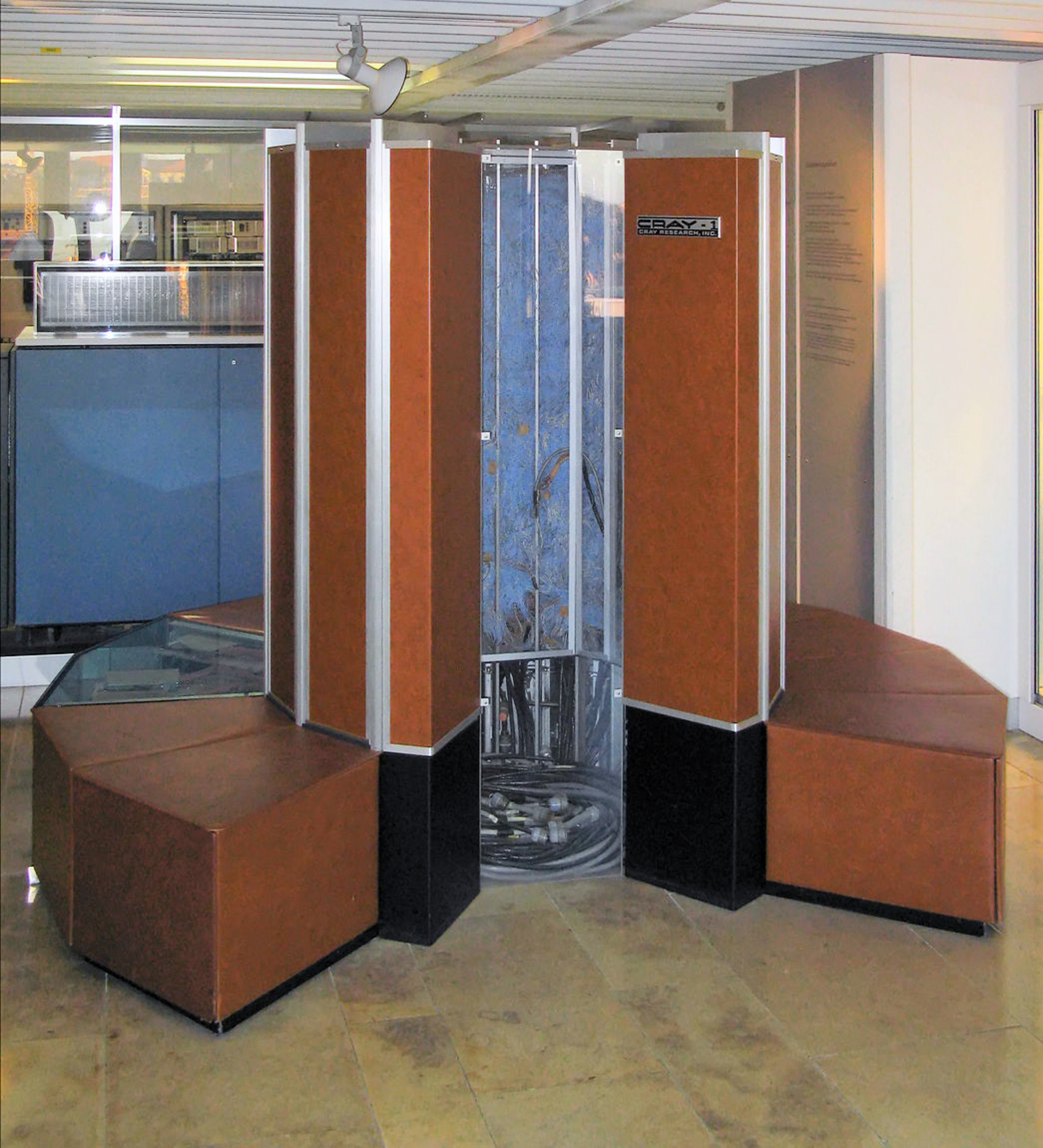
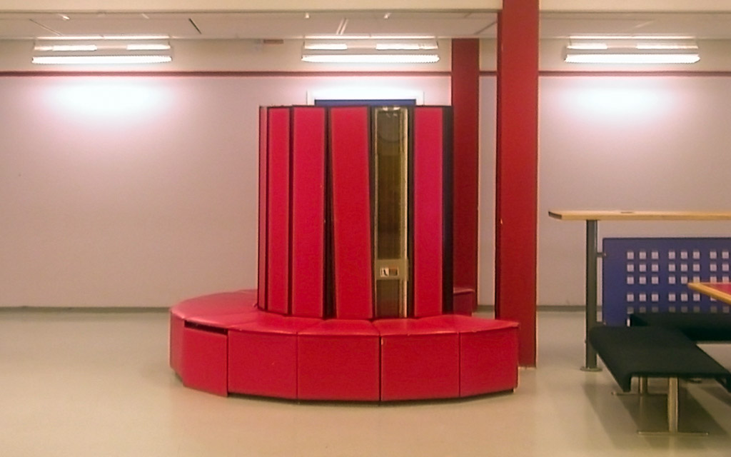
Our post on ECMWF ended on 24 October 1978, when Cray-1A serial number nine arrived by lorry at the gates of an unfinished building on the campus of the United Kingdom Meteorological Office’s Shinfield Park complex at Reading. The machine had been ordered in late 1976 against three competing bids from CDC and IBM; it was the first Cray-1 ever delivered to a customer in Europe; it had cost approximately eight million United States dollars in 1978 currency, paid by the sixteen founding member states of the European Centre. Nine months later, on 1 August 1979, it ran the Centre’s first operational global ten-day weather forecast on a 1.875-degree grid-point primitive-equation model at fifteen sigma vertical levels.
What that post left unresolved was: what did the Centre choose to run on that Cray-1A once the procurement was settled? The grid-point N48 model of 1979 was the bootstrap product. The serious operational forecasting that ECMWF would become known for began in April 1983, when the Centre switched its dynamical core from the grid-point N48 to a spectral T63L16 – and the spectral lineage it adopted ran not from any European centre but from the Australian Bureau of Meteorology Research Centre’s predecessor units in Melbourne, via the papers of a man who had visited Reading several times in the late 1970s but never accepted a permanent post there. The spectral method that took over ECMWF in 1983 was a method that, six years earlier, had been a peripheral Australian curiosity. The story of how it travelled from Melbourne to Reading – and to Princeton, and to Boulder, and to Washington, and to Tokyo – is the story of how a numerical method becomes a global operational standard.
It begins with a problem that had defeated every major modelling group of the 1960s.
The pole problem
A regular latitude-longitude grid is the obvious way to discretise the sphere. Wrap rectangular cells onto the globe, give each a longitude and a latitude, run finite-difference operators between adjacent cells. It is what every general-circulation model from Mintz-Arakawa at UCLA to Smagorinsky’s Zodiac at GFDL did through the 1960s. The trouble is that meridians converge at the poles.
If the grid has 2.5 degrees of longitude between adjacent cells, the physical east-west spacing of two adjacent grid points is a · cos(φ) · Δλ, where a is the Earth’s radius and φ is latitude. At the equator that is about 278 kilometres. At 80 degrees north it is about 48 kilometres. At 89 degrees north – the row immediately below the pole – it is about five kilometres. The zonal spacing has collapsed by more than an order of magnitude over the last few degrees of latitude.
This wrecks the explicit-timestep budget. The Courant-Friedrichs-Lewy condition for an explicit advection scheme requires that the time step Δt satisfy roughly u · Δt / Δx ≤ C, where u is the maximum signal speed and C is an O(1) stability constant. For the primitive equations the relevant speed is that of gravity waves, around 300 metres per second. The whole model has to run at the time step set by the smallest Δx anywhere on the grid – which means, on a regular lat-lon mesh, at the time step set by the pole. With Δx of five kilometres and u of 300 metres per second, the time step has to be on the order of a few seconds, even though the equator could happily tolerate several minutes. This is the pole problem, and it dominated the practical design of gridpoint atmospheric models for the entire pre-spectral era.3
The standard workaround, pioneered by Yale Mintz and Akio Arakawa at UCLA in the mid-1960s, was polar filtering. Take a Fourier transform of each field along each high-latitude latitude circle, zero out (or damp) wavenumbers above a latitude-dependent threshold, and inverse-transform back. The short zonal wavelengths that the polar grid could not stably advect at a sensible time step get killed before they cause trouble. Mintz and Arakawa filtered the zonal mass-flux variables and the zonal pressure-gradient terms in their general-circulation model. The technique worked, in the sense that the model ran at a tolerable time step without exploding. But nobody loved it. It was non-physical: information was thrown away at high latitudes, exactly where the polar vortex and the stratospheric circulation needed to be preserved. It was not energy-conserving: Arakawa’s enstrophy-conserving Jacobian had been the great theoretical triumph of 1960s gridpoint work, and polar filtering quietly undid part of that. And it was operationally awkward: picking the cutoff was a black art, and the filter had to be retuned every time the grid changed.
The other workarounds were similar in spirit. Yoshio Kurihara’s 1965 paper in Monthly Weather Review, written at GFDL, defined a reduced grid that kept the rectangular structure away from the poles but reduced the number of longitudinal grid points per latitude row as one approached them, so that physical Δx stayed roughly constant. Some groups tried polar caps – different coordinate patches near each pole – or stereographic projections. All these schemes added bookkeeping complexity to finite-difference operators that were already painful to write. A scheme that was straightforward on a rectangular grid became a maintenance nightmare when neighbour relationships varied by latitude.
This was the state of the art at the end of the 1960s: gridpoint models on lat-lon grids with polar filtering, an architecture that worked but was philosophically ugly. Then a different community – fluid-dynamics theorists who had been playing with spectral methods for incompressible turbulence – arrived with a completely different idea.
Spherical harmonics
The cleanest way to think about spectral methods is by analogy with sound. A musical note from a violin contains a fundamental pitch plus a series of overtones, each at an exact multiple of the fundamental. Any periodic vibration in a single dimension – the air in an organ pipe, the displacement of a guitar string – can be written as a sum of such pure tones. Mathematicians call this a Fourier series: an arbitrary waveform decomposed into sines and cosines. The deep fact is that this decomposition is natural for periodic problems on a line. Sines and cosines aren’t an arbitrary choice; they are the building blocks the geometry of the line itself picks out.
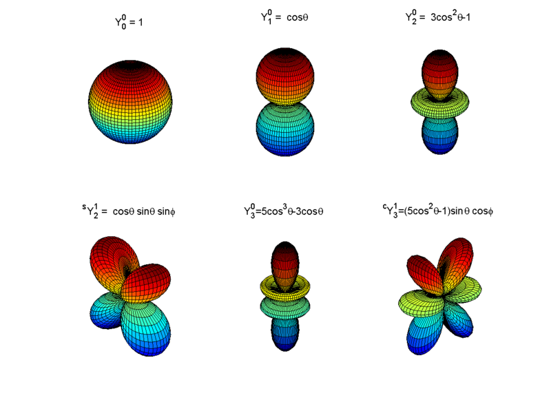
The same trick works on a sphere – it just needs a different family of building blocks. Instead of sines and cosines, the natural basis functions on the surface of a sphere are called spherical harmonics. They are the patterns of bumps and dimples that the sphere’s geometry singles out as fundamental: smooth global patterns indexed by two integers, the way piano keys are indexed by octave and note. One integer counts how many bumps run pole-to-pole; the other counts how many run east-to-west. The simplest spherical harmonic is just “a constant value everywhere on the globe.” The next few are two-lobed patterns (one hemisphere bright, the other dim), three-lobed patterns, four-lobed patterns, and so on, in a regular family. The figure below shows six representative members, drawn as three-dimensional bumps on a sphere.
Any meteorological field defined globally on the Earth – temperature, pressure, humidity, the wind in each direction – can be written as a unique sum of these spherical harmonics, each multiplied by its own coefficient. That sum is the spectral representation of the field. A weather model written in spectral form does not store gridded values of temperature; it stores spherical-harmonic coefficients, and reconstructs temperature on a grid only when it needs to.
Three properties of this basis matter for the rest of the story. The first is that the spherical harmonics treat every point on the sphere identically. There are no special points, no poles to give the model indigestion. The smooth bumps that make up the third spherical harmonic look the same near Antarctica as they do over the equator. The pole problem of the previous section simply does not arise. The second is that the harmonics are “orthogonal” in a precise mathematical sense – they do not contaminate each other when you take their sum. Adding more harmonics to a model is like adding more piano keys; the existing keys are unaffected. The third, more technical, is that the spherical Laplacian – the operator that governs how a field tends to smooth itself out, and that sits at the heart of gravity-wave propagation in the primitive equations – acts on each spherical harmonic by multiplication, not by mixing it with its neighbours. The Laplacian of a spherical harmonic of degree n is the same harmonic scaled by −n(n+1)/a², where a is the Earth’s radius. In gridpoint models, treating gravity-wave terms implicitly requires solving a giant coupled system of equations at every step. In spectral models, the same operation is a sequence of independent scalar divisions, one per coefficient. This single property, more than any other, is what made the semi-implicit time-integration scheme – which would later double or triple the affordable time step of every operational model – a natural fit for the spectral basis.
In practice a model cannot keep infinitely many spherical harmonics. It has to throw away the ones beyond some resolution cutoff. The choice of cutoff defines what the model can and cannot see. The modern standard is triangular truncation, written TN: keep every harmonic up to total wavenumber N and discard the rest. The “T” is for triangular, because if you plot the kept harmonics on a chart of pole-to-pole versus east-to-west wavenumbers, the kept set forms a triangle. The number N is the cutoff. The notation has stuck so well that the literature speaks of “running a T63 forecast” or “upgrading to T1279” the way one might speak of camera resolution. A rough rule of thumb for translating to gridpoint language: TN resolves features down to a half-wavelength of about 20 000 / N kilometres. So T63 corresponds to roughly 320-kilometre features, T1279 to roughly 16-kilometre ones. The progression from ECMWF’s first operational spectral model in 1983 to the present-day system runs from T63 to T1279 – a factor of about twenty in linear resolution, and roughly twenty thousand in computational cost. (NMC’s first operational spectral model, three years earlier, used the related rhomboidal truncation R30, which was the dominant North American convention in the late 1970s and early 1980s; the global convergence on triangular truncation came over the course of the 1980s, and NMC itself switched to triangular T80 in August 1987.)
The mathematical attraction of spherical harmonics for atmospheric simulation had been known since the 1950s. The first spectral barotropic experiment was due to the Princeton meteorologist Leonard Silberman in 1954.4 George Platzman at the University of Chicago published systematic studies of the truncated spectral vorticity equation in 1960 and 1962. The Canadian meteorologist André Robert, at McGill, did his 1965 doctoral thesis on the integration of the spectral barotropic vorticity equation on the sphere and published the result in the Journal of the Meteorological Society of Japan in 1966 – a paper that introduced both the systematic use of spherical-harmonic prognostic variables for an atmospheric model and the semi-implicit time-integration scheme that would later become a near-universal feature of operational models.5 Robert returned to the topic at the Tokyo IUGG/WMO symposium of 1969, where he laid out the semi-implicit treatment of gravity waves in a spectral framework.
The mathematics, in other words, was old. What had blocked the technique from operational adoption for fifteen years was a single computational obstacle, and it was severe enough that almost everyone working in operational forecasting had concluded the spectral method could not be made to scale to anything more interesting than a barotropic-vorticity toy.
The interaction-coefficient wall
The mathematics, in other words, was old. What had blocked the technique from operational adoption for fifteen years was a single computational obstacle. It was severe enough that almost everyone working in operational forecasting had concluded the spectral method could not be made to scale to anything more interesting than a barotropic-vorticity toy.
The problem was the non-linear terms. The equations of atmospheric motion contain products of unknown fields: the wind multiplied by the temperature gradient, the wind multiplied by itself, the pressure gradient times the density. Such products have to be evaluated at every time step. In gridpoint models the multiplication is trivial – you have the wind and the temperature at each grid point, you just multiply them together. In a spectral model, that trick is not available. The fields are stored as lists of spherical-harmonic coefficients, not as gridded values. Multiplying two spherical harmonics does not produce a third spherical harmonic; it produces a complicated mixture that has to be re-projected back onto the original basis.
The pre-1970 way of doing this was to precompute a giant lookup table, called the table of interaction coefficients, that tabulated exactly which combinations of three spherical harmonics produced overlap with which other harmonics. Every non-linear multiplication was then a weighted sum over this table. The trouble was the size of the table. The number of entries grew roughly as the sixth power of the truncation: doubling the resolution multiplied the cost by sixty-four. Even at the modest T20 resolution, the table strained the core memory of the largest computers of the late 1960s. At T40 or T60 it was simply hopeless. For any resolution remotely comparable to what gridpoint models were already achieving, the interaction-coefficient method ran out of both memory and time.
Silberman managed barotropic experiments. Platzman did systematic studies. But the interaction-coefficient method could not be pushed to high truncation, and certainly not to the full primitive equations on multiple vertical levels, because the cost grew like the sixth power of the resolution. This was the wall. By the late 1960s the consensus across the operational community was that spectral methods were elegant but operationally inaccessible – a research curiosity that the gridpoint community could safely ignore.
In 1970 two groups, working independently, on opposite sides of the Atlantic, on different journals, with different motivations, broke the wall in the same way.
The transform method
Both groups had the same insight: you do not have to evaluate the non-linear products in spectral space at all. You can transform the relevant fields to gridpoint space, multiply them pointwise where the multiplication is trivial, and transform back. The expensive interaction-coefficient sums in spectral space are replaced by an inverse transform, a pointwise multiplication on a grid, and a forward transform.
In June 1970 the American applied mathematician Steven Orszag, at the Massachusetts Institute of Technology, published “Transform method for the calculation of vector-coupled sums: Application to the spectral form of the vorticity equation” in the Journal of the Atmospheric Sciences.6 Orszag was a pure-applied-mathematics person with a background in incompressible-turbulence simulation; the paper treats the barotropic vorticity equation as a generic spectral problem in three-dimensional vector coupling. The mathematical argument is clean. The motivation is not particularly meteorological.
In the same year the Copenhagen group of Erik Eliasen, Bennert Machenhauer, and Erik Rasmussen, at the University of Copenhagen’s Institute for Theoretical Meteorology, published Report No. 2 of the Institute – a technical report, never offered to a journal – titled “On a numerical method for integration of the hydrodynamical equations with a spectral representation of the horizontal fields.” The Copenhagen report is famously hard to obtain; copies survive in physical archives. But it is universally cited as one of the two foundational papers of the transform method, and it is more practically oriented than the Orszag paper – explicitly aimed at numerical weather prediction rather than at fluid-dynamics theory.
The algorithm is straightforward to describe in retrospect. The model carries the atmospheric fields as lists of spherical-harmonic coefficients. At every time step it does three things. First, spectral to grid: it reconstructs the actual gridded fields from the coefficients, using a fast Fourier transform in the east-west direction and a related transform (the Legendre transform) in the north-south direction. Second, multiply on the grid: it performs the non-linear multiplications – wind times temperature, wind times wind, all the products that the equations of motion call for – as pointwise multiplications between gridded values, where the work is trivial. Third, grid to spectral: it transforms the products back into spherical-harmonic coefficients, again using FFTs and Legendre transforms.
This three-step dance replaces the interaction-coefficient lookup with an alternation between two representations of the same atmosphere. The atmosphere itself never changes. The model just looks at it differently at different points in the time step: as a list of harmonics when it needs to take spatial derivatives (which are trivial in spectral form) or apply the implicit gravity-wave operator (which is diagonal in spectral form), and as gridded values when it needs to multiply things together (which is trivial on a grid).
The cost saving was extraordinary. The interaction-coefficient method had grown like the sixth power of the resolution; the transform method grew roughly like the cube. At ECMWF’s T63 resolution of 1983, the transform method was about 250 000 times cheaper per time step. At T213 of the early 1990s it was roughly 100 million times cheaper. The transform method did not just improve the spectral approach – it made spectral primitive-equation models possible.
Orszag and Eliasen-Machenhauer-Rasmussen had broken the wall. What remained was the engineering problem of getting the transform method to work not for the barotropic vorticity equation but for the full multi-level baroclinic primitive equations that operational forecasters actually needed. That problem was substantially harder than the wall-breaking insight itself. And the man who solved it was not at Princeton, or at Boulder, or at the European Centre’s then-future Reading site. He was in Melbourne.
Bourke 1972, Bourke 1974
The Commonwealth Meteorology Research Centre had been established in 1967, on paper, and became operational in 1969 as a joint Bureau-CSIRO research unit in Melbourne. It was created by William James “Bill” Gibbs, Director of the Bureau of Meteorology from 1962 to 1978, and C. H. B. (Bill) Priestley, Chief of the CSIRO Division of Meteorological Physics at Aspendale, to give Australian numerical weather prediction a stable institutional home that bridged operational forecasting and basic atmospheric research. The model was explicit: Gibbs and Priestley wanted a small Melbourne unit that could do the kind of work Smagorinsky’s group did at Princeton, von Neumann’s at the Institute for Advanced Study, Mintz-Arakawa at UCLA. Its founding Officer-in-Charge, from 1969 to 1973, was Gilbert Brian “Brian” Tucker, born in Ogmore Vale in South Wales in 1930, who had graduated from Aberystwyth in 1950 and taken a doctorate in dynamical meteorology at Imperial College London in 1954. After RAF forecasting service and nine years as a research scientist at the United Kingdom Met Office, Tucker had been recruited to Melbourne in 1965 to become Assistant Director (Research and Development) of the Bureau, and was transferred to CSIRO in 1969 to take charge of the new joint centre.7
William Bourke – a research scientist whose biographical record before his publications is largely silent in the open documentary trail, and who is not to be confused with the unrelated William Meskill Bourke of the Australian Dictionary of Biography (a Labor and DLP politician, 1913-1981) – was attached to CMRC from the late 1960s onwards. He had visited GFDL with Barrie Hunt in the early 1970s, where they had together “originally worked out the spectral modeling techniques” in Stouffer’s later recollection.1 He wrote his first foundational paper from his desk in Melbourne. It is worth quoting the citation in full, because the institutional affiliation has been muddled in much subsequent literature, and the present series tries to keep these things precise:
Bourke, W. (1972). An efficient, one-level, primitive-equation spectral model. Monthly Weather Review 100(9): 683-689. Affiliation: Commonwealth Meteorology Research Centre, Melbourne.8
This is a CMRC paper, not an ANMRC or BMRC paper. ANMRC was the renamed CMRC of 1974, and BMRC did not exist until 1985. Pinning Bourke’s foundational work to the institution that actually produced it matters because so much of the secondary literature, including some otherwise excellent retrospectives, has the wrong acronym attached.
The 1972 paper is short by modern standards – seven pages. What it did, technically, is the following. It formulated a one-level (barotropic, but with mass continuity and a free surface, so closer to shallow-water than to pure barotropic-vorticity) global primitive-equation model on the sphere. Its prognostic variables were vorticity and divergence, not the velocity components u and v: this is the key trick, because on a sphere u and v have a coordinate singularity at the poles, while vorticity and divergence do not. All fields were expanded in spherical harmonics with triangular truncation. Non-linear advection terms were evaluated by the transform method of Orszag and of Eliasen-Machenhauer-Rasmussen. The time integration used André Robert’s semi-implicit scheme of 1969, which time-averages the linear gravity-wave terms so that the time step is no longer bound by the gravity-wave Courant-Friedrichs-Lewy condition but only by the much gentler advective one – a 3× to 6× speedup on its own. Integrations of 116 days were carried out. Energy, angular momentum, and squared potential vorticity were conserved to a high degree.
The abstract is unusually blunt for a Monthly Weather Review paper of the period: “the computational efficiency of the model is found to be far superior to that of an equivalent model based on the traditional interaction coefficients.”8 It was. The 1972 paper proved, on a working code on real machines, that the transform method could be made to drive a primitive-equation spectral model conservatively over month-long integrations. The remaining engineering question was whether the same idea would scale to many vertical levels – to the baroclinic atmospheres that operational forecasters actually had to deal with.
Two years later Bourke produced the answer. The CMRC had by then been renamed – after a 1973 internal review, the centre became formally independent of both parent agencies, reporting to CSIRO and to the Department of Science, and was renamed the Australian Numerical Meteorology Research Centre (ANMRC).9 Bourke’s affiliation on the 1974 paper is therefore ANMRC. The citation:
Bourke, W. (1974). A multi-level spectral model. I. Formulation and hemispheric integrations. Monthly Weather Review 102(10): 687-701. Affiliation: Australian Numerical Meteorology Research Centre, Melbourne.
The 1974 paper extended the transform machinery from one level to many – from a barotropic to a baroclinic atmosphere. This is non-trivial. It forces explicit handling of vertical advection, hydrostatic balance, and the thermodynamic energy equation in spectral space, with the semi-implicit treatment of the linearised gravity-wave operator now being a global elliptic problem at every step. On a grid the elliptic problem requires an iterative solver; on a spectral basis it diagonalises completely, because the Laplacian is diagonal on spherical harmonics. The semi-implicit method and the spectral basis paired with such mathematical naturalness that, in retrospect, it is hard to see them as separable. The 1974 paper demonstrated stable hemispheric integrations of the multi-level system, initialised from real Southern Hemisphere analyses. It introduced divergence damping as a practical fix for spurious large-scale inertia-gravity oscillations during model spin-up – a device that became operationally standard. For most subsequent reviewers, the 1974 paper is the operational-grade date stamp of spectral primitive-equation modelling. The model in the paper is recognisably the dynamical-core architecture of every spectral operational model that followed for the next four decades.
Three months later in the same calendar year, in the Quarterly Journal of the Royal Meteorological Society, Brian Hoskins and Andrew Simmons at the University of Reading published the parallel formulation that would become the European reference: “A multi-layer spectral model and the semi-implicit method,” QJRMS 101: 637-655 (1975).10 The Hoskins-Simmons paper is technically very close to Bourke 1974. The standard scholarly attribution is to cite both: Bourke 1974 in the Southern Hemisphere lineage, Hoskins-Simmons 1975 in the UK-and-ECMWF lineage, with the understanding that the two formulations were independent and contemporary. Hoskins-Simmons is, in places, more thorough on the analysis of stability and dispersion properties; Bourke is the one with the working operational-grade code. The pair is the standard founding citation for multi-level spectral NWP.
Honest priority claims
It is worth pausing to be clean about credit before the rest of the story takes off, because both the popular and the in-house retrospectives have a tendency to compress the history into “Bourke invented spectral NWP” – which is not true and which Bourke himself, on the evidence of his own 1988 review chapter and his 2021 historical paper on the Australian computing pioneers, would not have claimed.
Spherical harmonics for atmospheric modelling were not Bourke’s. Silberman 1954 was the first spectral barotropic experiment; Lorenz 1960 and Platzman 1960, 1962 followed; Robert 1966 was the first systematic application of spherical harmonics to NWP on the sphere with semi-implicit machinery; Robert 1969 introduced the semi-implicit time integration that Bourke 1972 then used. Robert’s work, done at McGill and the Recherche en prévision numérique (RPN) of the Canadian Meteorological Service in Dorval, gave the operational community its first spectral model in routine operation – a barotropic and shallow-water system that went operational in Canada around 1974, before Bourke’s multi-level paper was even in print. Canada was the first country to put a spectral algorithm into operational forecasting, by all the conventional accountings of operational adoption.11 What Canada had was an operational shallow-water spectral, however; not yet a multi-level baroclinic operational spectral.
The transform method was not Bourke’s. Orszag 1970 and Eliasen-Machenhauer-Rasmussen 1970 invented it, simultaneously and independently. Bourke used it.
What Bourke did, between 1972 and 1974, was to weld these existing components – spherical harmonics, the transform method, semi-implicit time integration, and the vorticity-divergence formulation of the primitive equations – onto a complete multi-level baroclinic model on the sphere, in working code, on the relatively modest computing of the CMRC in Melbourne, and to demonstrate that the resulting model conserved its quadratic invariants over month-long integrations. He was the first to show, on a working operational-grade code, that the whole stack could be made to fit together. Hoskins and Simmons did the same thing independently in Reading a year later. The two papers became the founding pair.
A clean framing: Robert provided the harmonics, Orszag and Eliasen et al. provided the transform, Bourke welded them onto the multi-level primitive equations with a stable semi-implicit time scheme and ran them long enough to prove the physics. Hoskins and Simmons did the same independently. The papers are the founding documents of operational spectral NWP. Robert had the first operational spectral model in any form, in Canada in 1974, but Robert’s was shallow-water; Bourke’s was the first multi-level baroclinic formulation in print.
Why Melbourne, of all places
The CMRC story tends to puzzle readers from larger institutional cultures, and the puzzle deserves to be named. By any straightforward measure of size or resources, Australian atmospheric science in 1969 was small. The Bureau of Meteorology was the operational forecasting agency of a country of twelve million people on the geographic periphery of the developed world. CSIRO Aspendale’s Division of Meteorological Physics had been founded in 1946 by C. H. B. Priestley, but it was a modest research unit. The CMRC, founded into this institutional context, employed dozens of people, not hundreds. Why did the dominant operational numerical method of 1983-2010 get invented at this peripheral Southern Hemisphere centre rather than at NCAR, GFDL, ECMWF, or the UK Met Office?
Several institutional answers, none sufficient on its own.
First, the Southern Hemisphere drove a different research agenda. Australia is operationally responsible for forecasting the weather of the Southern Hemisphere, which has very different geometry from the Northern: vast oceans south of the Tropic of Capricorn, almost no observational coverage south of New Zealand and South Africa, and an Antarctic continent that closes off the southern polar cap rather than opening it as the Arctic Ocean does. The pole problem on a latitude-longitude grid is, of course, formally symmetric between hemispheres. But the South Pole is a continent. Realistic model topography, especially of the Antarctic ice sheet, has to be represented exactly where the gridpoint geometry is at its worst. Spectral methods finesse this entirely – the spherical-harmonic basis is uniform on the sphere; there is no pole problem to begin with. For a centre with operational responsibility for the whole Southern Hemisphere down to and including Antarctica, that geometric uniformity was not just aesthetic. It was useful.
Second, the small-centre advantage. CMRC and ANMRC employed dozens of people, most of them focused on a single global model. That meant short feedback loops, no committee-driven model-development politics, and freedom to bet everything on one numerical approach. GFDL, NCAR, NMC and the UK Met Office all had to support multiple model lineages and broader research programmes. A small centre could pivot harder, on less consensus, and the consequence of getting it wrong was less institutionally costly because there were fewer parallel groups whose work would have to be unwound.
Third, Tucker’s protection. As a UK-Met-Office-trained dynamicist who had spent nine years inside a national weather service, Tucker understood the operational side’s pull toward immediate forecast improvement, and he understood that you have to fence off basic-research time deliberately or it evaporates. The ANMRC’s 1974 reorganisation as an independent unit, reporting to CSIRO and to the Department of Science rather than to the Bureau’s operational chain, was precisely such a fence. Bourke and his colleagues did not have to justify spectral methods in terms of next week’s operational forecast skill. They had time to do the thing.
Fourth, existing intellectual links to the UK and the US. Tucker came from the UK Met Office. Priestley had come from the UK before that. The Australian community read Monthly Weather Review and the Journal of the Atmospheric Sciences as their core journals; they did not need to cross any Pacific to be visible in the AMS literature. Bourke’s 1972 paper landed in MWR because that was simply where one published serious NWP work. The “Pacific crossing” the story can sometimes be told as is, on closer inspection, mostly an illusion – there was never a Pacific gap to cross, because the Australian community already treated the AMS journals as its natural home.
What Australia did not have was world-class computing. The literature does not give a clean machine list for CMRC and ANMRC in 1968-1985, but the general picture is that Bourke did his foundational work on modest computers by 1972 standards – Cybers and IBMs, certainly not Crays. Australia’s first dedicated NWP supercomputer was the NEC SX-4 installed at the joint Bureau-CSIRO High Performance Computing Centre at 150 Lonsdale Street in Melbourne in September 1997, almost a quarter-century after the foundational papers. The spectral method’s computational efficiency – its small constant factor for global integrations on limited-memory machines – was, for Australian computing, not just an aesthetic advantage. It was a necessity.
Puri carries the code
The 1972 and 1974 papers were the founding documents. The propagating object across the operational community, however, was not a paper. It was a piece of working code.
Some time after the 1974 paper appeared in print, Kamal Puri – a CMRC and then ANMRC research scientist who had taken his physics doctorate at the University of Manchester, and who had co-authored Bourke’s 1974 paper on horizontal resolution and the 1977 Methods in Computational Physics chapter – visited the National Center for Atmospheric Research at Boulder, Colorado, on an extended scientific exchange. He brought a copy of the Australian spectral model with him. He adapted it to NCAR’s computers. NCAR was running a CDC 7600 through 1977 and a Cray-1 from July 1977; the model was ported to one and then the other.
The NCAR Community Climate Model documentation describes the lineage precisely: “the original versions of the NCAR Community Climate Model, CCM0A and CCM0B, were based on the Australian spectral model (Bourke et al., 1977).” Puri did the porting at NCAR; Eric Pitcher (then at the University of Miami) and Robert Malone (at Los Alamos and the Department of Energy) subsequently modified the model further with NCAR-specific physics packages. The first CCM was released as a community-supported model in 1983.12 CCM0B evolved into CCM1 in 1987, CCM1 into CCM2 in 1992, and the spectral-dynamics lineage continued through CCM3 (1996) and CCM4 (1998) before being replaced by the Community Atmosphere Model (CAM) of 2004 and – in the architectural pivot of the late 2000s – by the CAM Spectral Element (CAM-SE) of CESM 1.0 (2010), which kept the spectral-element flavour but moved off the global Legendre transforms and onto a cubed-sphere mesh. For a quarter-century, every CCM and CAM run at NCAR and at the dozens of US university climate-research groups that depended on the community model carried the architectural DNA of the Australian spectral model that Puri had ported in the late 1970s.
The corresponding GFDL story is shorter on documented details but has Stouffer’s testimony to anchor it: “In the mid-1970s, GFDL imported a copy of the spectral GCM code developed by W. Bourke.” Holloway at GFDL then bolted Smagorinsky’s Manabe-era Zodiac physics onto Bourke’s dynamical core, producing the GFDL Supersource model that ran at GFDL into the 1990s.1 The Princeton laboratory that had defined finite-difference atmospheric modelling under Smagorinsky and Manabe, the lineage of the Zodiac and Markfort codes, was therefore running its 1970s and 1980s spectral GCM on code that had been written in Melbourne. This is the most striking institutional moment in the propagation history.
What both the NCAR and the GFDL adoption stories illustrate is the propagation mechanism. Numerical methods become operationally dominant not principally through their founding papers, even when the founding papers are landmarks. They become dominant when a working reference implementation crosses laboratory boundaries and is adopted, adapted, and ported elsewhere. The 1972 and 1974 MWR papers told the world that the method could be made to work. The Australian code, carried by Puri and by other visitors, was what other centres actually built on. Methods propagate as artifacts – as working code – more than as papers. This is the post’s thesis, and it will recur in the chronology that follows.
The Cray symbiosis
The reason the spectral transform method became, in the late 1970s and early 1980s, the architectural choice of every major operational forecasting centre is also the reason it would eventually be replaced: it was an almost perfect fit for the vector-pipelined supercomputers of its era.
Look at the operations in the transform method, as itemised in the preceding sections. There is an FFT along each latitude row – an O(N log N) cascade of butterfly operations on a contiguous vector. The Cooley-Tukey FFT is the canonical textbook vector workload. There is a Legendre transform – a matrix-vector multiplication of a precomputed Legendre table against a vector of zonal coefficients, one product per zonal wavenumber. Matrix-vector is also a clean vector pattern: long inner products with no data dependencies between elements. There are pointwise multiplications in gridpoint space – trivially vectorisable: load two arrays, multiply, store. And there are inverse transforms of the same shape as the forward ones.
There is no stencil operation in the inner loop. There is no branch logic. There is no data-dependent indirection. The entire inner loop of a spectral transform model is one long sequence of matrix-vector multiplies and FFTs. This is the architecture every vector machine ever made was designed to do well.
The arrival of the Cray-1 at NCAR in July 1977 and at ECMWF on 24 October 1978 was, looked at from the spectral-method side, a precisely-timed accident. Bourke had published the multi-level transform model in 1974. Cray Research delivered the first machine that could run it at operational scale, anywhere outside a national laboratory, a few years later. The Cray-1’s headline performance – peak 250 megaflops, sustained around 138 megaflops, twelve-and-a-half-nanosecond clock – depended on its eight 64-element vector registers and chained vector pipelines. The machine could load, multiply, and add streams of floating-point operands in a steady pipeline if the data were laid out as long, contiguous vectors. It could not extract much performance from short loops, scattered memory access patterns, or stencil operations that hopped between non-contiguous arrays.
The canonical contemporary benchmark, frequently cited from the Cray-1 architecture overview of the period, was a 64-point Fast Fourier Transform: roughly 47 milliseconds in scalar mode on a CDC 7600, dropping to about 3 milliseconds on the Cray-1 in vector mode, a factor of about fifteen.13 More broadly, vectorising a typical scientific code yielded speedups in the range 2.5× to 10× on the same Cray-1 hardware, depending on how cleanly the inner loops mapped onto vector operations. The Cray-1 was, in vector mode, five times faster than the CDC 7600 that NCAR had been running since 1977 – the figure that justified the $8.86 million procurement.
A finite-difference primitive-equation model evaluates spatial derivatives by referencing grid neighbours: (u[i+1,j] − u[i−1,j]) / (2Δx). The inner loop touches three arrays at three offsets. On a Cray-1 of the late 1970s, this caused several pain points. There was no cache; register reuse was hard when each iteration moved on to new neighbours. Stencils that stepped in the j direction accessed memory at large strides, which was slow on banked-memory vector machines. Polar filtering, when present, broke vectorisation entirely – the filter was a row-dependent operation that interrupted the steady stream of vector operations. A finite-difference model could be made to perform reasonably on a Cray, but it needed careful hand-tuning and the speedup over scalar mode was typically modest.
The spectral model vectorised almost on first writing. That asymmetry – spectral codes running near peak on vector hardware that the finite-difference codes were not designed for – is what gave the spectral transform method its decisive operational edge through the late 1970s and the entire 1980s. Vector machines were almost the only commercially available supercomputers for atmospheric science in that period: Cray-1, Cray X-MP, Cray Y-MP, Cray C90, the Japanese NEC SX series, the Fujitsu VP series. All of them were optimised for the same workload shape. All of them favoured the spectral transform method. By the early 1980s every operational global model of consequence had gone spectral.
The operational map of the 1980s
The first major operational adoption after the foundational papers was NCEP. The American National Meteorological Center at Suitland, Maryland – predecessor of today’s NCEP – had been running primitive-equation gridpoint models on its IBM 360/195s through the 1970s. Joseph Sela began spectral-model development at NMC in 1975, working from the Bourke 1974 paper and the Hoskins-Simmons 1975 companion. Sela’s first operational global spectral model, a rhomboidal R30 truncation at twelve sigma vertical levels, went into production in August 1980 on the NMC IBM 360/195s, supplemented as the decade progressed by Cyber and Cray hardware.14 (The model had entered the parallel Global Data Assimilation System cycle on 27 May 1980; the operational AVN and MRF forecast products switched to it in August.) The NCEP spectral lineage that began on that August 1980 day – the descendants of Sela’s R30L12, upgraded to R40L12 on the Cyber 205 in October 1983 and converted to triangular truncation T80L18 in August 1987 – continued in operation, with steadily increasing resolution and steadily updated physics, until 12 June 2019, when GFS version 15 replaced the spectral dynamical core with the FV3 finite-volume cubed-sphere core developed at GFDL. The spectral GFS served the National Weather Service for thirty-eight years, eleven months, and three weeks.
The second major operational adoption was ECMWF, on 30 April 1983, when the Centre’s grid-point N48 model was replaced by a T63 spectral model at sixteen sigma vertical levels. The switchover was on the same Cray-1A serial number nine that had been running the grid-point model since 1979. The implementation drew principally on the Hoskins-Simmons formulation and on the work of Cliff Temperton, then at ECMWF, who built the Centre’s spectral-transform infrastructure – the FFTs and Legendre transforms – to run efficiently on Cray vector hardware. Bourke was a frequent visiting scientist at the Centre through 1976-1980 but never accepted a permanent post there; his papers, and the implementation knowledge he had brought via Reading visits and via NCAR contacts, were the propagating mechanism. The Centre upgraded from the Cray-1A to a Cray X-MP/22 in 1984 and to a Cray X-MP/48 in December 1985, running the spectral model at progressively higher throughput on each generation.2
The third major operational adoption was JMA, the Japan Meteorological Agency. Masao Kanamitsu – then at JMA Tokyo, later at NCEP, finally at the Scripps Institution of Oceanography – led the team that built JMA’s first operational global spectral model. The work was published in 1983 in the Journal of the Meteorological Society of Japan: Kanamitsu, Tada, Kudo, Sato, and Isa, 1983, “Description of the JMA operational spectral model,” J. Meteor. Soc. Japan 61(6): 812-828.15 The model was T42 at twelve vertical levels initially, growing with each subsequent system upgrade. JMA’s first formally operational spectral GSM cycle (GSM8911) entered production in November 1989, although the development version had been running experimentally since 1983. JMA’s spectral GSM lineage stayed operational, with steadily increasing resolution, until well into the late 2010s.
By the mid-1980s the spectral method had effectively taken over operational global numerical weather prediction. Météo-France developed ARPEGE jointly with ECMWF – the two models share large fractions of their code base and are, in some sense, the same model run in different configurations – with ARPEGE going operational at Météo-France in 1992. The Deutscher Wetterdienst experimented with spectral methods but eventually went a different way (the ICON system of 2015, which we will come to). NCAR’s CCM line dominated US academic climate modelling on the spectral side. GFDL’s Supersource ran spectral dynamics for Manabe-era climate runs into the 1990s. The Bureau of Meteorology in Melbourne – Bourke’s institutional home – finally moved its own operational global forecasting onto a fully spectral system in the early 1990s, with the Global Assimilation and Prediction (GASP) system that descended directly from Bourke’s 1974 paper. Australia was first to invent operational multi-level spectral NWP and late to deploy it operationally – a typical pattern for small national centres, where the research lead is real but the operational rollout lags.
The resolution ladder
The chronology of operational resolution increases at ECMWF – which kept the cleanest public record of any of the operational centres – is the standard spine for the spectral era. Each upgrade was tied to the next supercomputer purchase. The progression telegraphs the architectural relationship between the method and its hardware:
| Truncation | Approx. grid spacing | Operational from | Machine class |
|---|---|---|---|
| T63L16 | ~210 km | 30 April 1983 | Cray-1A / Cray X-MP/22 |
| T106L19 | ~125 km | May 1985 | Cray X-MP/48 |
| T213L31 | ~63 km | September 1991 | Cray Y-MP and Cray C90 era |
| TL319L60 | ~40 km (ensemble) | 1999 | Fujitsu VPP700 |
| TL511L60 | ~40 km (HRES) | 21 November 2000 | IBM POWER4 cluster era |
| TL799L91 | ~25 km | 1 February 2006 | IBM POWER5 cluster |
| TL1279L137 | ~16 km | 26 January 2010 | IBM POWER7 cluster |
| TCo1279L137 | ~9 km | 8 March 2016 | Cray XC30/XC40 |
“TL” denotes the linear reduced Gaussian grid (Hortal and Simmons 1991 – see below), “TCo” the cubic octahedral grid (Wedi 2014 – also see below). The factor-of-twenty resolution increase from T63 in 1983 to TCo1279 in 2016 corresponds to a roughly twenty-thousand-fold increase in computational cost per forecast, broadly tracking Moore’s law over the same thirty-three years.
Two innovations along the ladder are worth singling out because both pushed the spectral method’s operational lifespan further than it would otherwise have run, and both reflect engineering responses to specific computational pathologies of the basic method.
The first is the reduced Gaussian grid of Manuel Hortal and Andrew Simmons at ECMWF, published in MWR 119: 1057-1074 (April 1991).16 The Gaussian grid required by the Legendre transform places the same number of longitude points on every latitude. On the sphere this clusters grid points near the poles – the same problem the lat-lon grid had, but now redundant rather than singular: the polar grid points carry no information that the spherical-harmonic truncation can resolve. Hortal and Simmons demonstrated that one could reduce the number of longitude points per latitude row near the poles, provided the discrete Fourier transform along each row still resolved the longest zonal wave at that latitude, with no loss of accuracy and a 20-25% saving in computational time and storage at T106. The technique was implemented operationally at ECMWF immediately and has been retained ever since.
The second is the octahedral cubic grid of Nils Wedi at ECMWF, published in Phil. Trans. R. Soc. A 372: 20130289 (2014).17 By the 2010s the linear reduced Gaussian grid had drifted out of optimal balance: the spectral truncation was being matched against a gridpoint resolution somewhat coarser than the spectral content required, producing spectral blocking and aliasing artefacts. Wedi proposed two simultaneous changes. The first was a cubic grid – use N+1 gridpoints to represent N waves, eliminating aliasing of triple products. The second was an octahedral arrangement – a reduction rule based on inscribing an octahedron in the sphere, producing a more uniform physical grid spacing than the conventional Hortal reduction. The combined “TCo” grid went operational at ECMWF on 8 March 2016 with IFS cycle 41r2.17 The O1280 octahedral grid has roughly 20 per cent fewer points than the equivalent N1280 reduced grid, with the same spectral resolution and improved fidelity at small scales.
There is one further development that extended the spectral method’s operational viability by perhaps two decades and that should at least be named here, although it deserves its own post: the marriage of spectral dynamics with semi-Lagrangian advection. André Robert again – “A stable numerical integration scheme for the primitive meteorological equations,” Atmosphere-Ocean 19: 35-46 (1981) – demonstrated that a semi-Lagrangian treatment of advection (trace each grid point’s air parcel back along a trajectory to its location at the previous time step) is stable for Courant numbers significantly greater than one. Combined with the semi-implicit treatment of gravity-wave terms that Bourke and Hoskins-Simmons had built in, the semi-Lagrangian semi-implicit (SLSI) scheme gave stable integrations with time steps four to six times longer than the corresponding Eulerian semi-implicit model. Andrew Staniforth and Jean Côté’s 1991 review in MWR 119: 2206-2223 consolidated the technique. By the early 1990s every operational spectral model had adopted semi-Lagrangian advection. The SLSI spectral model could run with time steps an order of magnitude longer than an explicit gridpoint model at the same resolution, which more than compensated for the somewhat higher per-step cost of the spectral transforms. This is the architectural reason that spectral models continued to dominate operational NWP through the 1990s, even after the parallel-scaling problems we will turn to had begun to become visible.
What the Gaussian grid actually looks like
It is worth pausing briefly on the physical-space side of the spectral picture, because the way the spectral transform method “lives” on a Gaussian grid is the visual entry point that makes the rest of the story concrete.
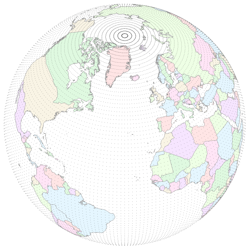
The Gaussian grid is, in a sense, the spectral method’s quiet compromise with finite arithmetic. Spherical harmonics are infinite-dimensional; the Legendre transform between physical and spectral spaces requires integration over latitude; Gauss-Legendre quadrature gives an exact integration rule for that latitude integral using a finite set of points placed at the roots of an appropriately chosen Legendre polynomial. Those roots are not equally spaced; they cluster slightly toward the poles. The longitude points on each Gaussian latitude row are equally spaced – the FFT along the row needs them to be – but the latitudes themselves are not. The “T62” or “T63” or “TL799” label specifies a spectral truncation; the implied Gaussian grid is the physical-space mesh that the truncation is exactly integrated on. Every spectral model alternates, twice per time step, between the spectral basis (where derivatives and the elliptic problem are trivial) and the Gaussian grid (where non-linear products are trivial). The two spaces are equivalent up to the truncation. The transform method is the bridge.
The contrast with a lat-lon grid is sharp.

The Gaussian grid solves the pole problem because the spherical-harmonic basis it serves was never embarrassed by the poles in the first place. The grid is a finite-arithmetic shadow of an underlying continuous basis whose only privileged geometry is the sphere itself. This is the architectural property that makes the spectral method natural on the sphere – the only reason, ultimately, it was worth the engineering work to get the transform method functioning.
The counter-currents
It is important not to tell the spectral story as if every operational centre went over to it. Two large counter-currents ran through the 1980s and 1990s and they deserve to be named.
The first is the UK Met Office’s Unified Model. The Met Office began the Unified Model programme in 1990 and went operational with it in June 1991. The Unified Model was – and is – a gridpoint model on an Arakawa C-grid in rotated lat-lon coordinates. The Met Office, the institutional descendant of the British meteorological tradition that had produced Reading-side spectral work through Hoskins-Simmons and Andrew Simmons (who had moved from Reading to ECMWF in 1979), did not itself go spectral operationally. This is sometimes told in retrospect as a deliberate hedge against the parallel-scaling problems of spectral methods, but the contemporary literature suggests the actual motivation was unification: running the same dynamical core globally, regionally, and at limited-area scales is structurally easier in a gridpoint framework, because limited-area spectral methods are messy. The parallel-scaling argument was retrospective. By the time the parallel-scaling cliff actually arrived in the 2000s, the Met Office was well-placed by accident.
The second is the GFDL move away from spectral for comprehensive coupled climate work. Even after the mid-1970s code import from Australia – the Supersource model – GFDL eventually moved off spectral for its flagship coupled-climate runs. The reasons given in GFDL’s own retrospectives are two: Gibbs ringing in topography (spherical harmonics struggle to represent the sharp edge of a mountain without ringing artefacts in the orographic forcing), and difficulty conserving the mass of tracers and dry air to machine precision over the long climate integrations that matter for chemistry transport and for centennial-scale runs.18 GFDL’s eventual replacement was the FV3 – the finite-volume cubed-sphere dynamical core whose development through the 2000s positioned it to become NCEP’s operational core in 2019.
Spectral was never universal. It was operationally dominant – which is a softer and more accurate claim than “operationally universal.” The two largest counter-currents were the Met Office’s institutional preference for unified gridpoint dynamics and GFDL’s institutional preference for long-run coupled-model mass conservation. Both choices look prescient in retrospect. Neither was straightforwardly about HPC architecture at the time.
The cluster era
The transition that would prove decisive for the spectral method’s operational lifespan was a hardware transition. It did not happen all at once. It is most easily marked by the slow displacement of vector supercomputers by massively-parallel commodity clusters across the 1990s and early 2000s – a transition that ECMWF’s procurement history records precisely. The Cray Y-MP and Cray C90 of the late 1980s and early 1990s were the last canonical register-vector machines at ECMWF. The Fujitsu VPP700 of 1996-2001 was a parallel vector system, halfway between architectures. The IBM POWER4 and POWER5 and POWER7 clusters of 2001-2010 were no longer vector machines at all. They were distributed-memory clusters of (eventually) thousands of scalar processors connected by a fast interconnect.
The spectral transform method has one mathematical property that makes it perfect for vector machines and devastating for distributed-memory clusters: the Legendre transform is global in latitude. To compute the coefficient a_{n,m} from gridpoint data, one must integrate against P_n^m(sin φ) over all latitudes. Every latitude row contributes to every spectral coefficient that has a non-trivial Legendre weight there. Operationally this means: if the gridpoint data are decomposed across MPI ranks by latitude bands, the forward Legendre transform requires every rank to communicate its partial sums to every other rank that holds a coefficient. This is an all-to-all communication pattern – the hardest pattern to scale to large core counts.
The standard parallel implementation, developed at ECMWF and at NCEP through the 1990s, is the transposition strategy: rather than communicate within each transform, fully redistribute the data between successive stages (gridpoint → Fourier coefficients → spectral coefficients) so that each transform is local to a single rank. This works. But every transposition is an all-to-all on the whole grid, and all-to-all communication time grows roughly as O(P log P) or worse in the number of MPI ranks P.
The arithmetic is what then drives the architectural pivot. When P is small – a few hundred MPI ranks, which was the operational scale through the early 2000s – the all-to-all is cheap and the spectral method wins on raw floating-point cost. When P is large – many thousands of ranks – the all-to-all begins to dominate. At about ten thousand cores the spectral transform method begins to lose. At a hundred thousand cores it is structurally uncompetitive against well-designed local-stencil schemes. The crossover happened during the 2010s, on commodity clusters of progressively larger core counts.
The methods that won the architectural pivot all share the same property: operations are local in space. Each grid cell talks only to its few immediate neighbours. Parallel decomposition is then trivial – split the mesh into patches, give one patch to each rank, exchange ghost cells with neighbours, and the model scales linearly.
The dominant local-stencil candidates were three. Finite-volume on a cubed sphere: GFDL’s FV3, developed through the 2000s and ultimately chosen by NCEP for GFSv15 in 2019. Finite-volume on an icosahedral mesh: DWD’s ICON, operational 20 January 2015, jointly developed with the Max Planck Institute for Meteorology in Hamburg.19 Spectral element on a cubed sphere: NCAR’s CAM-SE, an evolution of the spectral lineage that retains the spectral basis but applies it on quadrilateral elements of a cubed-sphere mesh rather than on global spherical harmonics, eliminating the global Legendre transform; operational in CESM 1.0 from 2010.

The closing brackets
The closing brackets of the spectral era are easy to enumerate.
20 January 2015: DWD’s ICON goes operational, replacing the spectral GME model that had run at DWD since 2001. Icosahedral finite-volume dynamics; full local-stencil parallelism. ICON was the first operational system at a major centre to be designed from the outset for petascale and exascale architectures.
8 March 2016: ECMWF’s TCo1279 octahedral cubic grid goes operational with IFS cycle 41r2. This is the spectral method’s hybridised survival strategy. The dynamics are still spectral. The grid is now quasi-uniform on the sphere, which lets the gridpoint stages of the transform method parallelise better and slightly extends the spectral method’s operational lifespan. The Wedi 2014 paper that motivated it is titled, with characteristic candour, “Increasing the horizontal resolution in numerical weather prediction and climate simulations: illusion or panacea?”17 ECMWF was, by this point, openly skeptical of how much further the spectral method could be pushed.
12 June 2019: NCEP retires the operational spectral GFS, replacing it with GFS version 15 built on the FV3 finite-volume cubed-sphere core developed at GFDL. The Sela spectral lineage that had begun in August 1980 ended after thirty-eight years, eleven months, and three weeks of continuous operational service. The replacement was, in a sense, the institutional return: GFDL had imported Bourke’s spectral code in the mid-1970s, run it for two decades as Supersource, and was now exporting the finite-volume code that displaced spectral methods at the largest American operational centre.
By 2026, the operational map is mixed. NCEP runs FV3. DWD runs ICON. The Met Office is migrating from the UM to LFRic, on a cubed-sphere mesh built around a finite-element discretisation, with the LFRic programme started in 2011. NCAR has CAM-SE in CESM and MPAS on icosahedral mesh for the next generation. The Bureau of Meteorology in Melbourne – Bourke’s institutional home – moved off its own spectral GASP system in the late 2000s, adopting the UK Unified Model under the ACCESS programme. Australia, which had been first to invent operational multi-level spectral NWP, was an early adopter of its replacement. The Japan Meteorological Agency, which had been one of the first operational spectral systems in the early 1980s, has been pivoting through the late 2010s and into the 2020s.
ECMWF stands alone among the major centres in still using the spectral transform method as its operational dynamical core. The TCo1279 hybrid grid has carried it for the decade after 2016. ECMWF’s research programme is openly experimenting with IFS-FVM, a finite-volume reformulation of the IFS that ran in research configurations from 2019 onwards.20 The institutional working assumption is that ECMWF will eventually move off the global spectral transform method too, though no operational switchover date has been announced as of 2026.
Spectral dynamics did not so much die as get cornered. The era of universal operational use ran from August 1980, when NCEP went operational with Sela’s R30L12, to June 2019, when NCEP went off the spectral GFS for FV3 GFSv15 – a thirty-eight-year window almost exactly bracketed by the operational dominance of vector and then early-cluster supercomputing. The Cray-1 of 1976 to the Cray X-MP, Y-MP, C90 of the 1980s and early 1990s were the vector-supercomputer era proper. The Cray T3D and T3E of the mid-1990s were the start of the parallel-cluster era. The IBM POWER and Cray XC and modern Xeon and GPU systems of the 2000s and 2010s were the era in which the spectral method’s parallel-scaling problems became operationally decisive. Spectral was, very nearly, the architectural method of vector supercomputing. Both reigned together. Both retreated together.
Coda
William Bourke is, as of 2026, almost certainly still alive. He published a substantial historical paper as recently as 2021 in the Proceedings of the Royal Society of Victoria: “Pioneering of numerical weather prediction in Australia: Dick Jenssen, Uwe Radok and CSIRAC,” Proc. R. Soc. Victoria 133(2): 67-81.21 The paper recovers a 1957-1959 episode – early Australian barotropic experiments on the CSIRAC vacuum-tube computer, work that had been buried in a thesis – and offers it to a wider scientific community. It is in some respects an instructive choice of valedictory project for someone whose own work fifty years earlier launched the dominant operational numerical method of three decades. The Bourke of 2021 is, on the evidence of that paper, someone who cared about institutional and intellectual memory: he chose to write up other people’s pioneering work, not his own.
The numerical method he and his colleagues welded together in 1972 and 1974 outlived its hardware era by perhaps fifteen years – the cluster-era survival of spectral methods at ECMWF, the cushioning effect of the semi-Lagrangian time-step extension, the reduced and octahedral Gaussian grids that mitigated the worst of the parallel-scaling pathology. The shape of the curve, however, is clean. The method was born on a Cray. It propagated through the vector-supercomputer era as the natural workload of that hardware. When the hardware era ended, the method’s home advantage evaporated. Code that took fifteen years to write took two decades more to retire, even after the architectural pivot had been declared. By 2019 the largest operational deployment had been retired. By the late 2020s the spectral method is, as of writing, a residue at one major centre rather than a universal practice. A clean rise-and-fall arc, marked at both ends by the architecture of the supercomputers that ran the code.
There is one durable lesson in the propagation story that ought to outlive the method itself. Methods do not become operationally dominant principally through the papers that describe them. They become operationally dominant when a working reference implementation – code that runs, that converges, that conserves the right invariants, that produces a usable forecast on real hardware – crosses laboratory boundaries and is adopted, adapted, and ported elsewhere. The 1972 and 1974 Monthly Weather Review papers are the founding documents of operational spectral NWP. They are the things that students of the field read in graduate seminars. But the propagating object was the Australian spectral code that Kamal Puri carried to NCAR, that someone unnamed carried to GFDL, and that Cliff Temperton, Adrian Simmons, and others at ECMWF re-implemented from scratch but built around the Bourke-Hoskins-Simmons formulation. The reference implementations were what changed the operational landscape. The papers were the warrant.
Posts in this series have made the related claim about other numerical methods and other hardware eras: the Mintz-Arakawa lineage propagated through codes at UCLA and at GFDL; the Cane-Zebiak ENSO model propagated through a basement VAX in 1986; the TOGA-TAO observing array propagated through Argos satellite uplinks and shared data products. What propagates is not the idea. What propagates is the artifact that makes the idea cheap to copy. Code propagates. Papers describe.
Footnotes
-
Edwards, P. N., A Vast Machine: Computer Models, Climate Data, and the Politics of Global Warming (MIT Press, 2010), online supplement, GFDL chapter, at https://pne.people.si.umich.edu/vastmachine/i.GFDL.html, citing personal communication from Ronald Stouffer, 13 May 1998. Note that Edwards conflates the Commonwealth Meteorology Research Centre (CMRC, 1969-1974) with the Australian Numerical Meteorology Research Centre (ANMRC, 1974-1984) – Bourke’s home institution at the time of the original spectral work was CMRC. ANMRC succeeded CMRC only in 1974. ↩ ↩2 ↩3
-
For ECMWF’s institutional history through the Cray-1A and the 1983 spectral switchover, see our post on First Cray in Europe. The April 1983 switchover from grid-point N48 to spectral T63L16 ran on the same Cray-1A serial number nine that had been running the gridpoint model since 1 August 1979. ↩ ↩2
-
For a modern restatement of the pole problem and the family of workarounds, see Bénard, P. (2019), “An assessment of global numerical weather prediction at the pole,” Quart. J. Roy. Meteor. Soc. 145, and Williamson, D. L. (2007), “The evolution of dynamical cores for global atmospheric models,” at https://www.gfdl.noaa.gov/bibliography/related_files/jlh7301.pdf. ↩
-
Silberman, L. (1954), “Planetary waves in the atmosphere,” Journal of Meteorology 11: 27-34. ↩
-
Robert, A. J. (1966), “The integration of a low order spectral form of the primitive meteorological equations,” Journal of the Meteorological Society of Japan 44: 237-244. Robert’s 1969 semi-implicit paper was presented at the Tokyo IUGG/WMO symposium on numerical methods in atmospheric models. The text of Robert 1966 is in the public record at https://www.atmos.albany.edu/facstaff/rfovell/ATM562/robert-1966.pdf. ↩
-
Orszag, S. A. (1970), “Transform method for the calculation of vector-coupled sums: Application to the spectral form of the vorticity equation,” Journal of the Atmospheric Sciences 27: 890-895. At https://journals.ametsoc.org/view/journals/atsc/27/6/1520-0469_1970_027_0890_tmftco_2_0_co_2.xml. Eliasen, E., Machenhauer, B., and Rasmussen, E. (1970), “On a numerical method for integration of the hydrodynamical equations with a spectral representation of the horizontal fields,” Report No. 2, Institut for theoretisk meteorologi, University of Copenhagen. ↩
-
For Tucker’s biographical and institutional record, see EOAS “Tucker, Gilbert Brian (Brian)” (P003315) and CSIROpedia, “Gilbert Brian Tucker [1930-2010].” ↩
-
Bourke, W. (1972), “An efficient, one-level, primitive-equation spectral model,” Monthly Weather Review 100(9): 683-689. The AMS journal record is at https://journals.ametsoc.org/view/journals/mwre/100/9/1520-0493_1972_100_0683_aeopsm_2_3_co_2.xml. ↩ ↩2
-
For the CMRC → ANMRC → BMRC sequence and the associated governance reorganisations, see Encyclopedia of Australian Science entries at https://www.eoas.info/biogs/A000912b.htm and https://www.eoas.info/biogs/A000913b.htm. The 1974 reorganisation made ANMRC formally independent of both parent agencies, with the Officer-in-Charge “responsible to the CSIRO and the Secretary, Department of Science.” ↩
-
Hoskins, B. J., and Simmons, A. J. (1975), “A multi-layer spectral model and the semi-implicit method,” Quart. J. Roy. Meteor. Soc. 101: 637-655. The Wiley record is at https://rmets.onlinelibrary.wiley.com/doi/10.1002/qj.49710142918. ↩
-
For Robert’s role in Canadian operational spectral NWP, see the CMOS Bulletin tribute, “André Robert: One of the very first scientists to successfully perform a simulation of the atmosphere’s general circulation at the global scale using a computer model,” at https://bulletin.cmos.ca/andre-robert-one-of-the-very-first-scientists-to-successfully-perform-a-simulation-of-the-atmospheres-general-circulation-at-the-global-scale-using-a-computer-model/. ↩
-
For the NCAR CCM0A/CCM0B lineage and the explicit attribution to the Australian spectral model, see the NCAR CCM technical notes (notes 187, 317, 382, and 400 in the NCAR/TN series), at https://opensky.ucar.edu/system/files/2024-08/technotes_187.pdf and https://opensky.ucar.edu/system/files/2024-08/technotes_400.pdf. The 1977 review chapter that the CCM0A documentation cites is: Bourke, W. P., McAvaney, B., Puri, K., and Thurling, R. (1977), “Global modelling of atmospheric flow by spectral methods,” in Methods in Computational Physics 17, ed. J. Chang (Academic Press), pp. 267-324. ↩
-
The 47 ms scalar / 3 ms vector benchmark figures for a 64-point FFT on the Cray-1 are from contemporary Cray Research architecture documentation, summarised in the Cray-1 overview at http://www.openloop.com/education/classes/sjsu_engr/engr_compOrg/spring2002/studentProjects/Andie_Hioki/Cray1withAdd.htm. The comparison is between scalar and vector modes on Cray-1 / contemporary CDC hardware; care should be taken with rhetorical framing. ↩
-
Sela, J. (1980), The NMC Spectral Model, NOAA Technical Report NWS 30. The Hathitrust catalogue record is at https://catalog.hathitrust.org/Record/102347136. The NCEP retrospective on GFS history, including the 12 June 2019 transition to FV3 GFSv15, is in the NOAA press release at https://www.noaa.gov/media-release/noaa-upgrades-us-global-weather-forecast-model and in the AMS 2019 retrospective on the GFS. ↩
-
Kanamitsu, M., Tada, K., Kudo, T., Sato, N., and Isa, S. (1983), “Description of the JMA operational spectral model,” Journal of the Meteorological Society of Japan 61(6): 812-828. At https://www.jstage.jst.go.jp/article/jmsj1965/61/6/61_6_812/_article. Kanamitsu was at JMA Tokyo at the time, later at NCEP, and finally at Scripps. There is no joint Kanamitsu-Bourke paper; the simultaneous adoption of the spectral transform method at JMA and at the Australian Bureau in the early 1980s was the consequence of two groups working from the same published literature, not of direct institutional collaboration. ↩
-
Hortal, M., and Simmons, A. J. (1991), “Use of reduced Gaussian grids in spectral models,” Monthly Weather Review 119(4): 1057-1074. The AMS record is at https://journals.ametsoc.org/view/journals/mwre/119/4/1520-0493_1991_119_1057_uorggi_2_0_co_2.xml. ↩
-
Wedi, N. P. (2014), “Increasing the horizontal resolution in numerical weather prediction and climate simulations: illusion or panacea?”, Philosophical Transactions of the Royal Society A 372: 20130289. At https://royalsocietypublishing.org/doi/10.1098/rsta.2013.0289. The ECMWF IFS cycle 41r2 release notes documenting the 8 March 2016 TCo1279 operational implementation are at https://confluence.ecmwf.int/display/FCST/Detailed+information+of+implementation+of+IFS+cycle+41r2. ↩ ↩2 ↩3
-
The GFDL model-history page lays out the reasons for moving away from spectral dynamics for comprehensive coupled climate work: https://www.gfdl.noaa.gov/brief-history-of-global-atmospheric-modeling-at-gfdl/. The reasons cited are Gibbs ringing in topography and difficulty conserving mass to machine precision for long climate runs. ↩
-
Zängl, G., Reinert, D., Rípodas, P., and Baldauf, M. (2015), “The ICON (ICOsahedral Non-hydrostatic) modelling framework of DWD and MPI-M: Description of the non-hydrostatic dynamical core,” Quart. J. Roy. Meteor. Soc. 141: 563-579. At https://rmets.onlinelibrary.wiley.com/doi/10.1002/qj.2378. ↩
-
For ECMWF’s IFS-FVM research programme as the contemplated successor to the spectral IFS, see the IFS-FVM description paper in Geoscientific Model Development 12: 651 (2019), at https://gmd.copernicus.org/articles/12/651/2019/gmd-12-651-2019.pdf, and the ECMWF retrospective “Fifty years of Earth system modelling at ECMWF” at https://www.ecmwf.int/sites/default/files/elibrary/81651-fifty-years-of-earth-system-modelling-at-ecmwf.pdf. ↩
-
Bourke, W. (2021), “Pioneering of numerical weather prediction in Australia: Dick Jenssen, Uwe Radok and CSIRAC,” Proceedings of the Royal Society of Victoria 133(2): 67-81. At https://www.publish.csiro.au/RS/RS21010. ↩