Jagadish Shukla’s memoir, A Billion Butterflies, devotes a chapter to each of the seven generations of digital computer he used between 1962 and 2024. The chapter sequence – paper and slide rule at Banaras Hindu University, IBM 360/65 at MIT, Texas Instruments Advanced Scientific Computer at the Geophysical Fluid Dynamics Laboratory, IBM 360/91 and CDC Cyber 205 and Cray X-MP at NASA Goddard, Convex C220 at the University of Maryland, Beowulf-pattern Linux clusters at the Institute of Global Environment and Society, distributed cloud at George Mason University – is the architectural history of supercomputing across sixty years told from the seat of one user. We covered Shukla and his career arc in the previous post. This post pulls the same seven-generation frame out of one career and lays it across the whole NWP-history series.
The argument is simple. Each architectural generation allowed atmospheric scientists to pose a specific kind of question that the previous generation could not. The hardware did not just make the science faster; it made different science possible. The 1922 forecast that Lewis Fry Richardson worked out by hand and pencil, in the rear of an ambulance unit in northern France, was correct in conception but produced answers six hours late and several thousand kilopascals wrong. The 1950 forecast that Jule Charney, Ragnar Fjørtoft, and John von Neumann ran on the ENIAC in Aberdeen Maryland was the same conception, but produced answers an hour faster than the actual weather and approximately right. The difference was not the conception. It was the machine. This post is about how the machines changed, and what each change made tractable.
Era 1: Vacuum tubes and the first forecast (1946-1958)
The first electronic digital computers were vacuum-tube machines: ENIAC (1946, University of Pennsylvania, eighteen thousand vacuum tubes, forty by eight by three feet, 150 kilowatts), EDVAC (1949), SEAC (1950, US National Bureau of Standards), Whirlwind I (1951, MIT, four thousand tubes), UNIVAC I (1951, Eckert-Mauchly), and the IAS machine (1952, Princeton’s Institute for Advanced Study, designed by John von Neumann). The architectural pattern was uniform: thousands of vacuum tubes acting as switching elements, a memory of approximately one thousand words (initially in mercury delay lines, then in Williams tubes, then – starting at Whirlwind in 1953 – in magnetic core memory, the architectural step that we covered in our post on Whirlwind I), and a central processor running at approximately one hundred kilohertz with single-instruction-per-cycle scalar arithmetic.
The atmospheric science that this hardware allowed was bounded by the memory. A forecast model in 1950 needed to fit its grid points, its half-dozen state variables per grid point, its handful of physics parameterisations, and its programme code into approximately one thousand words of total memory. The original ENIAC forecast of April 1950 used a two-dimensional barotropic model – a single layer of atmosphere, no vertical structure, on a fifteen-by-eighteen grid of approximately seven hundred kilometres horizontal resolution covering most of North America. The model produced one forecast in approximately twenty-four hours of ENIAC running time. By 1953 the same conception, on more capable hardware, was producing forecasts faster than the weather. The architectural transition from mercury delay lines to magnetic core memory at Whirlwind in 1953 was the load-bearing change: core memory had a one-microsecond access time, was non-destructive, and was the first computer memory technology that could store the kilobytes of state that an atmospheric model needed without dominating the machine’s cycle time.
What it allowed: the first numerical weather forecast (Post 9 in this series), the first non-trivial atmospheric simulation, and the institutional birth of operational numerical weather prediction at the US Joint Numerical Weather Prediction Unit at Suitland Maryland in 1954-1958. The Joint Unit ran on an IBM 701 (Post 14) and produced daily 36-hour forecasts that, on average, were better than the official manual forecasts of the United States Weather Bureau by 1958. The first principle of computational meteorology was established: a digital computer could forecast the weather better than a trained human meteorologist if you gave it enough memory and a reasonable atmospheric model. That principle has not been overturned in seventy-six years.
What it could not do: it could not handle the third dimension. Vertical resolution – the structure of the atmosphere from surface to stratosphere – was beyond the memory budget of vacuum-tube machines. The first quasi-three-dimensional climate model, Norman Phillips’s February 1956 Quarterly Journal of the Royal Meteorological Society paper “The general circulation of the atmosphere: A numerical experiment” (Post 7), used five kilobytes of total memory and ran on the Princeton IAS machine for thirty-three days of wall clock time. Phillips’s model had two atmospheric layers and a hemispheric grid. It worked. But it was at the upper end of what vacuum-tube hardware could do.
Era 2: Discrete transistors and the first GCMs (1958-1968)
The shift from vacuum tubes to discrete silicon transistors was the technological hinge of the late 1950s. Transistors were three orders of magnitude smaller, drew three orders of magnitude less power, generated three orders of magnitude less heat, and – after the production processes matured around 1958 – were two orders of magnitude more reliable than vacuum tubes. The first commercial transistor-based computer of consequence to atmospheric science was the CDC 1604 of 1960 (Post 29), Seymour Cray’s first design at Control Data Corporation, of which serial number one was delivered to the Naval Postgraduate School at Monterey California for use by the Fleet Numerical Weather Center. The 1604 had a memory of approximately 32 768 forty-eight-bit words (about 200 kilobytes in modern reckoning), a clock cycle of approximately ten microseconds, and a peak rate of about 100 000 floating-point operations per second.
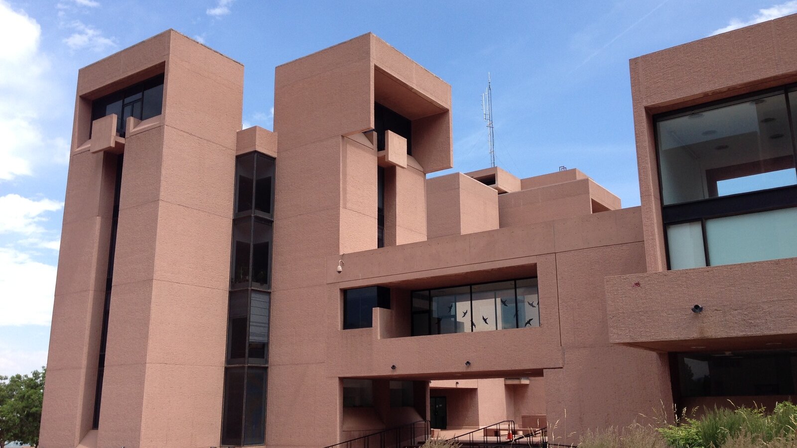
The 1962 IBM 7090 (Post 14) at the National Meteorological Center at Suitland was a contemporary – a transistorised re-implementation of the IBM 709 vacuum-tube architecture, with five times the throughput of its predecessor at one tenth the heat dissipation. The Joint Numerical Weather Prediction Unit at Suitland ran the 7090 alongside a 7094 from 1964 onwards. By 1965 the CDC 6600 (Post 30) was operating at the National Center for Atmospheric Research in Boulder, with serial number seven – ten times the performance of the 7090 and the canonical scientific supercomputer of the discrete-transistor era. The architectural step was: ten parallel functional units, each performing a different arithmetic operation, dispatched by a hardware scoreboard that tracked operand readiness. Three megaflops sustained, five and a half years of NCAR production use, and the platform on which Akira Kasahara and Warren Washington ran the first generation of the NCAR atmospheric general circulation model (Post 32).
What it allowed: the first true atmospheric general circulation models. By 1965 the atmospheric-modelling research programme could afford ten-layer hemispheric simulations on grids of approximately three hundred kilometres horizontal resolution, integrated over hundreds of simulated days. The Kasahara-Washington 1967 paper in Monthly Weather Review (covered in Post 32) was the foundational document. Syukuro Manabe and Kirk Bryan at GFDL (Post 16) ran their early coupled-model experiments on the UNIVAC 1108 through 1967-1973 – twelve hundred hours of compute per simulation. The first operational five-day forecast at NMC began regular production in 1962 on the IBM 7090. The discrete-transistor era was when atmospheric simulation moved from a research curiosity into an institutional discipline.
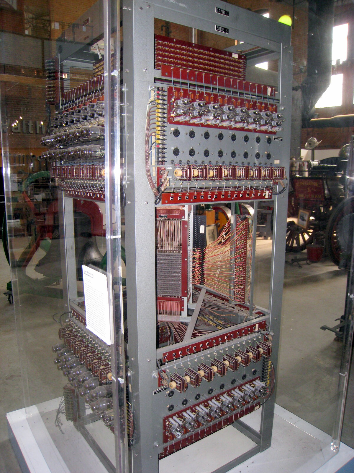
What it could not do: it could not handle ensembles. Each simulation took weeks of wall-clock time, and there was no spare compute for repeating an experiment with perturbed initial conditions. The Lorenz two-week predictability limit (Post 8), discovered by Edward Lorenz on a Royal McBee LGP-30 vacuum-tube-and-drum-memory machine in 1961, was understood as a fundamental limit by 1965. But quantifying its consequences for operational forecasting required ensemble experiments that the discrete-transistor era could not afford.
Era 3: Integrated circuits and the deep pipeline (1968-1975)
The shift from discrete transistors to integrated circuits – multiple transistors fabricated together on a single silicon die, with internal connections etched in metal layers – happened in two waves. The first wave, small-scale integration (SSI), packaged ten to a hundred transistors per chip and reached commercial atmospheric supercomputers around 1968-1970. The second wave, medium-scale integration (MSI), packaged hundreds to a few thousand transistors per chip and reached commercial machines around 1972-1975. The two waves together let computer designers build machines whose transistor counts had not been physically possible to wire by hand, and whose clock rates rose from the discrete-transistor era’s roughly ten megahertz to the integrated-circuit era’s roughly thirty-five megahertz.
The atmospheric machines of this era were the IBM System/360 Model 91 (Post 31), the CDC 7600 (Post 32), and the ILLIAC IV (Post 33). They embodied three different architectural philosophies. The 360/91 used Tomasulo’s algorithm for dynamic out-of-order scalar execution – a technique that would lie dormant for twenty-eight years before being revived in 1995 by Intel’s Pentium Pro and going on to become the universal organising principle of every modern central processing unit. The 7600 used deep pipelining of nine functional units under a simplified scoreboard, with a two-level main-memory hierarchy of small fast core memory and large slow core memory that was the conceptual ancestor of the modern cache hierarchy. The ILLIAC IV used sixty-four lockstep processing elements in a Single Instruction Multiple Data array – a philosophy that did not commercially work in 1975 but would, fifty years later, return as the modern graphics processing unit.
The 7600 was the workhorse of the era. Approximately seventy-five units were sold worldwide between 1969 and 1976. NCAR ran serial number twelve from May 1971 to April 1983 – almost twelve years – carrying the second generation of the Kasahara-Washington general circulation model and the early Community Climate Model through the start of the modern climate-modelling community. CERN ran a 7600 from February 1972 to 1984 doing high-energy physics event reconstruction. Lawrence Livermore National Laboratory ran four 7600s simultaneously through the 1970s for nuclear weapons design, networked together by the in-house Octopus wide-area network – the first large-scale supercomputer-cluster networking system in production use. Each architectural generation since has built on the patterns the 7600 established.
What it allowed: deep pipelining for atmospheric simulation, two-level memory hierarchies, and the first ensemble experiments. By 1980 NCAR could run a single ten-day forecast in a few hours of CDC 7600 wall-clock time. Cecil Leith’s 1974 Monthly Weather Review paper on Monte Carlo ensemble forecasting was theoretically possible because the underlying computations had become cheap enough to repeat with perturbed initial conditions. The architectural step from the discrete-transistor era’s “one simulation per week” to the IC era’s “ten simulations per day” was the precondition for Shukla’s 1981 Journal of the Atmospheric Sciences paper on monthly-mean predictability (Post 35) and for Tim Palmer’s eventual operational ensemble forecasting at ECMWF (Post 34).
What it could not do: medium-range forecasting at multinational scale. Each 7600 was an institutional asset and was time-shared among many users; no single weather service in 1975 had the budget for a 7600 of its own and a model big enough to outperform the existing operational models. The institutional bet that solved this problem – pool sixteen national budgets to buy a single shared facility – waited until the European Centre for Medium-Range Weather Forecasts opened operations in August 1979.
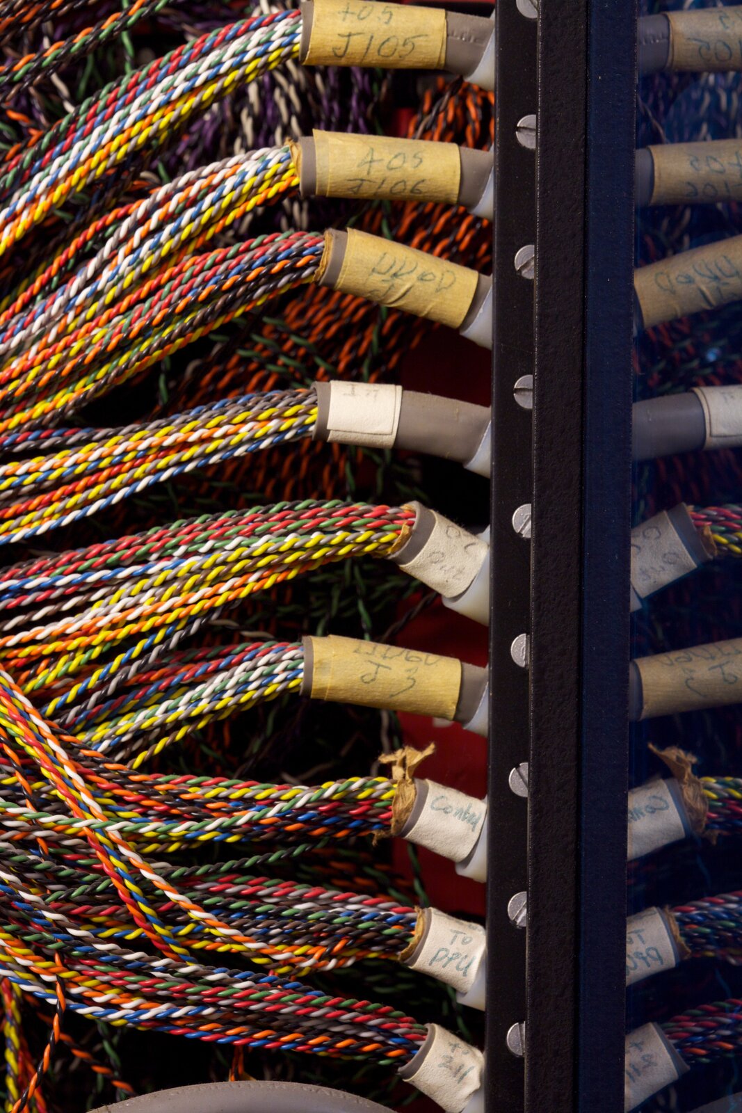
Era 4: LSI, ECL, and the Cray-1 (1975-1985)
The shift from MSI to large-scale integration (LSI) – ten thousand to a hundred thousand transistors per chip – happened around 1975-1980. The companion technological shift was from transistor-transistor logic (TTL) to emitter-coupled logic (ECL) integrated circuits, which switched in nanoseconds rather than tens of nanoseconds and let computer clock rates rise from the IC era’s thirty-five megahertz to the LSI era’s eighty megahertz. The atmospheric supercomputer that defined the era was the Cray-1 of 1976 (Post 26) – Seymour Cray’s first product at his eponymous Cray Research Inc., delivered to Los Alamos National Laboratory as serial number one on 4 March 1976, to NCAR as serial number three in July 1977, and to ECMWF as serial number nine on 24 October 1978 (Post 34).
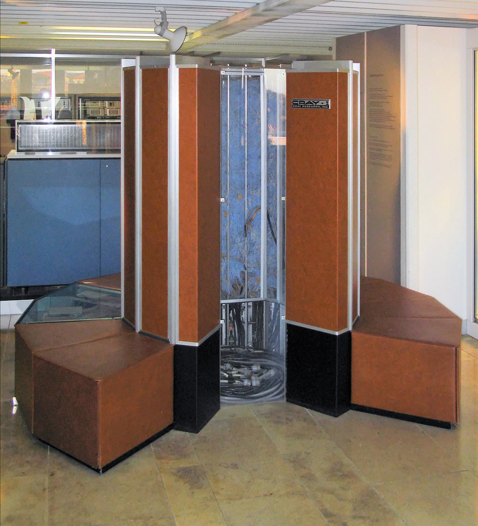
The Cray-1’s architectural innovation was the vector register: eight registers each holding sixty-four sixty-four-bit floating-point elements, into which long vectors of data could be loaded in a single instruction and operated on by deeply pipelined functional units at one element per clock cycle. The single-fast-memory model – one megabyte of fast core, no two-level hierarchy – deliberately abandoned the SCM/LCM scheme of the CDC 7600 in favour of letting the vector registers play the role of the cache. The Cray-1 sustained eighty megaflops on real atmospheric-model workloads, eight times the CDC 7600’s sustained rate, and was the platform on which the first generation of operational medium-range weather forecasting was built. Approximately eighty Cray-1 units were delivered between 1976 and 1982; the successor Cray X-MP (1983) and Cray Y-MP (1988) added shared-memory multiprocessing on the same architectural pattern and sold over two hundred units combined.
What it allowed: operational medium-range weather forecasting at the European Centre for Medium-Range Weather Forecasts (1 August 1979, ten-day global forecasts twice daily on a 1.875-degree grid-point primitive-equation model), doubling-of-CO2 climate sensitivity simulation at GFDL Princeton (Manabe-Wetherald 1975, Post 16), and the first generation of community climate models at NCAR. The atmospheric science that the Cray-1 generation enabled is the science that turned medium-range weather forecasting from a research aspiration into an operational discipline of every major national meteorological service.
What it could not do: ensemble forecasting at scale. A Cray-1 cost approximately eight million dollars in 1978 currency and was a single-user resource for any given forecast cycle. The five-hour Cray-1A wall-clock time per ten-day forecast at ECMWF in 1979 (Post 34) precluded running the same forecast a hundred times with perturbed initial conditions. Operational ensemble forecasting – which would become the universal pattern of medium-range and seasonal-to-interannual prediction – waited for cheaper machines.
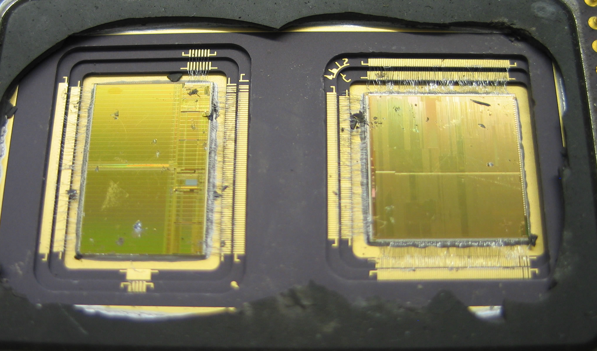
Era 5: VLSI and the personal supercomputer (1985-1995)
The shift from LSI to very-large-scale integration (VLSI) – a million transistors or more on a single chip – happened around 1985 and the resulting architectural shift was, in retrospect, the most consequential of the seven generations: the microprocessor went from being a low-end embedded controller to being the unit on which the entire computing industry was rebuilt. The MIPS R2000 (1985), Sun SPARC v7 (1986), Motorola 88000 (1988), and Intel 80486 (1989) were the first VLSI microprocessors fast enough to compete with traditional minicomputers on real scientific workloads. By 1990 a DEC VAX (Post 27) ran approximately ten megaflops sustained – one eighth the speed of a Cray-1 of 1976 – in a desk-sized cabinet at one twentieth the price.
The atmospheric science that VLSI allowed is captured precisely in the story of the Cane-Zebiak ENSO model (Post 27): Mark Cane and Stephen Zebiak’s 1985 coupled atmosphere-ocean model of El Niño-Southern Oscillation, designed at the Lamont-Doherty Earth Observatory and small enough to run on a single MicroVAX in approximately four hours per ENSO cycle. The Cane-Zebiak model produced the first successful operational forecast of an El Niño event in late 1986 – a forecast that was, on the day it was made, the first time that any team had successfully predicted an El Niño several months ahead. The model code was, at the time, considered too small to take seriously by the supercomputer-class climate-modelling community at NCAR and GFDL; the forecast went out anyway, and was correct, and changed the field.
What it allowed: personal climate computing. By 1990 a competent atmospheric scientist with a workstation in their office could run small-to-medium-scale models that, fifteen years earlier, would have required time on a Cray. The institutional pattern of atmospheric-science computing began to fragment: the operational forecasting centres stayed on big iron (ECMWF on Cray X-MP and Y-MP, NCEP on Cray and IBM, Met Office Bracknell on Cray) but the research community migrated, in fits and starts, to workstation-based personal computing. The 1981 Shukla framework (Post 35) for monthly-mean predictability could now be tested by individual research groups on workstations; the operational centres adopted the framework into seasonal forecasting through the 1990s; the seasonal-prediction discipline became, in this decade, fully operational.
What it could not do: ensemble forecasting at the scales that the Shukla framework needed. A workstation could run a single model, but running fifty workstations in parallel as a single distributed simulation was a software-engineering problem that the VLSI era did not solve. That problem waited for the cluster era.
Era 6: The cluster era (1995-2010)
The shift from individual workstations to clusters of workstations running a coordinated parallel computation was less an architectural shift than a software-and-systems-engineering one. The hardware – VLSI microprocessors, Ethernet networks, commodity disk drives – existed by 1990. The software stack that knitted them into a single computational substrate – Message Passing Interface (MPI) as the standard portable parallel-programming library, Linux as the standard operating system, the Beowulf cluster pattern as the institutional reference architecture – was assembled across 1992-1996. The defining moment was Beowulf-1, built in summer 1994 at the Center of Excellence in Space Data and Information Sciences at NASA Goddard by Donald Becker and Thomas Sterling: sixteen Intel 80486 DX4 processors at 100 MHz, 16 megabytes of DRAM each, two channel-bonded 10-megabit Ethernet networks, approximately five hundred megaflops aggregate. The 1995 Sterling-Savarese-Becker-Dorband-Ranawake-Packer paper “Beowulf: A Parallel Workstation for Scientific Computation” was the canonical reference.
Atmospheric science adopted the cluster pattern in two distinct waves. The first was institutional: Jagadish Shukla’s IGES-COLA (Post 35), founded January 1993, deliberately built its computing infrastructure on workstation clusters rather than Cray big iron, and was the first major climate-research centre to make that architectural choice operational. By 2000 the COLA cluster was running approximately five hundred Linux x86 cores; by 2005, two thousand cores. The second wave was the migration of the existing supercomputer-centre operational workloads onto cluster architectures: NCAR’s Cray architectures gave way through the early 2000s to IBM Power-based clusters (Bluefire, Yellowstone, Cheyenne, Derecho); ECMWF’s Cray T3D (1994) and Fujitsu VPP700 (1996) were intermediate steps that already used distributed-memory parallelism; by 2010 every major operational forecasting centre was running a cluster of some configuration.
What it allowed: ensemble climate modelling at the scales the Shukla framework needed. The 1992 ECMWF EPS (Post 34) on a Cray Y-MP could afford 33 ensemble members at T21 resolution; by 2010 cluster-based EPS systems were affording 51 members at T799 resolution – an improvement of approximately two thousand times in compute per ensemble member. The Coupled Model Intercomparison Project (CMIP), launched 1995 and providing the principal computational input to every Intergovernmental Panel on Climate Change Assessment Report from AR2 (1995) to AR6 (2021), was a community-distributed cluster-based experiment. By 2010 the IPCC consensus on anthropogenic climate change rested on hundreds of independently-developed climate models running on clusters at over fifty institutions in over twenty countries. None of this was possible on Cray big iron.
What it could not do: machine-learning-based forecasting at the scales that emerged in the late 2010s. The VLSI cluster could run the explicit physics-based models very well; what it could not do efficiently was train a deep neural network on decades of reanalysis data and use the trained network as a forecast model. That required a different architectural step.
Era 7: GPUs and the return of the SIMD philosophy (2010-)
The last architectural shift in this story is the rise of the graphics processing unit as a general-purpose scientific computing substrate. The shift began with NVIDIA’s G80 GPU of 2006 – the first commercially successful programmable GPU with a Single Instruction Multiple Thread architecture – and accelerated through the Tesla generation (2008-2010), the Fermi generation (2010-2012), the Kepler generation (2012-2014), and onwards through the Pascal, Volta, Ampere, Hopper, and Blackwell generations of 2016-2026. The architectural philosophy of the modern GPU is direct lineage from Daniel Slotnick’s ILLIAC IV of 1972 (Post 33) – many small processing elements operating in lockstep against many parallel data items, with per-element conditional masking. The ILLIAC IV had sixty-four processing elements at sixteen megahertz; the modern NVIDIA H100 has sixteen thousand eight hundred and ninety-six CUDA cores at 1.8 gigahertz. The architectural similarity is exact; the scale difference is two thousand and fifty times the processing elements at one hundred and twelve times the clock rate.
The atmospheric science that the GPU era allowed is, in 2026, an actively unfolding story rather than a settled history. Two threads are visible. The first is direct GPU acceleration of physics-based models: the European Centre for Medium-Range Weather Forecasts’ Integrated Forecasting System runs portions of its physics on GPUs from approximately 2020; the United Kingdom Met Office Unified Model is being ported to GPU through the late 2020s; NCAR’s MPAS and CESM models are GPU-accelerated. The architectural argument is the same as the 1976 Cray-1 vector argument, scaled up: atmospheric models consist of long sequences of identical operations across grid columns, which is the workload pattern GPUs are designed for.
The second thread is more disruptive: machine-learning-based forecasting models trained on reanalysis data. The 2022-2023 generation of ML forecast models – Pangu-Weather (Huawei, 2022), GraphCast (DeepMind, 2023), FourCastNet (NVIDIA, 2023), GenCast (DeepMind, 2024) – are GPU-trained neural networks that, on the medium-range forecasting benchmark, outperform the operational physics-based models of the major weather centres at one ten-thousandth the runtime cost per forecast. This is not a quantitative improvement on existing methods. It is a categorically new methodology, enabled entirely by GPU compute and forty years of accumulated reanalysis data. The 2024 ECMWF Annual Seminar identified ML-based forecasting as the principal disruptive technology of operational meteorology since the 1979 commissioning of ECMWF itself. The same architectural philosophy that did not produce weather on Slotnick’s ILLIAC IV in 1975 (Post 33) is now producing the most accurate weather forecasts in the world.
What it allowed: ML-based forecasting, subseasonal-to-seasonal prediction at scale, and the integration of operational forecasting with climate-research workflows that had previously been institutionally separate. What it disrupted: every prior architectural assumption about how atmospheric models should be designed, validated, and operationally deployed. The disruption is incomplete in 2026 and is the principal active research programme of the international atmospheric-science community.
What the Hardware Did
The architectural story across these seven eras can be summarised in one sentence: the questions that atmospheric scientists asked were the questions the available hardware could answer. Richardson’s 1922 forecast was the question vacuum-tube hardware would answer in 1950. Phillips’s 1956 climate model was the question discrete-transistor hardware would answer at NCAR and GFDL in the 1960s. Manabe’s coupled-model climate-sensitivity calculations of the 1970s were the question integrated-circuit hardware would answer on the TI ASC. Tim Palmer’s 1985 ensemble-forecasting concept was the question Cray-class hardware would barely answer in 1992 and that cluster hardware would comprehensively answer by 2005. Pangu-Weather and GraphCast in 2022-2023 are the questions that GPU hardware allowed.
Each architectural era had a distinctive operational rhythm that was set by the hardware. In the vacuum-tube era, a single forecast took twenty-four hours of wall-clock; the operational rhythm was “run yesterday’s forecast for tomorrow.” In the discrete-transistor era, the same model took two hours; the rhythm was “run today’s forecast for tomorrow’s weather and yesterday’s verification.” In the integrated-circuit era of the CDC 7600, a ten-day forecast took five hours; the rhythm was “run two operational forecasts a day plus research overnight.” In the Cray-1 era at ECMWF, the same five-hour rhythm scaled to twenty national meteorological services on one machine. In the cluster era, the rhythm became “run an ensemble of fifty forecasts twice a day, on one machine, with research workflows running in parallel on the same cluster.” In the GPU era, the rhythm has become “run a continuously-updated ensemble plus an ML inference for cheap real-time forecasts.” The operational rhythm of weather forecasting has tracked the operational rhythm of the underlying hardware with a tightness that is unusual in the history of computational science.
The architectural step that did not happen is also worth noting. The vector philosophy – one fast scalar processor with deeply pipelined functional units, plus vector registers to hide memory latency – won the 1976-1995 commercial supercomputer market, and the SIMD philosophy – many small processors operating in lockstep against many parallel data items – lost. By 2026 the verdict has been substantially reversed: SIMD is the dominant architectural philosophy of the modern GPU and the modern machine-learning compute substrate, while vector pipelining survives as a side-feature on every modern central processor without dominating the market. Cray’s 1976 architectural bet won the commercial market for thirty years. Slotnick’s 1972 architectural bet won the commercial market for the next thirty years. Both philosophies, in retrospect, were correct on different timescales. The lesson is that architectural history is not, in general, monotonic.
The Human Side
Across these seven eras the institutional pattern of atmospheric-science computing also changed. In the vacuum-tube era, every major numerical weather prediction effort was a partnership between two or three named individuals – Charney, Fjørtoft, von Neumann; Phillips alone; Lorenz alone – working at a research institution that had built or acquired one machine. By the discrete-transistor era, the operational forecasting centres (NMC at Suitland, the UK Met Office at Bracknell, the Soviet Hydrometeorological Center at Moscow) were running computer-supported operations with staffs of dozens. By the integrated-circuit era, the research-supercomputer centres (NCAR, GFDL, Lawrence Livermore, CERN) had hundreds of staff. By the LSI/Cray-1 era, the European Centre for Medium-Range Weather Forecasts – founded in 1973 by sixteen European states pooling their meteorological-computing budgets – was an institution with hundreds of staff serving the operational needs of dozens of national weather services. By the cluster era, the Coupled Model Intercomparison Project was a distributed community of thousands of scientists across over fifty institutions in over twenty countries, all running independently-developed models on independently-procured hardware and contributing to a shared scientific consensus. By the GPU era, the principal atmospheric-science institutions are augmented by several technology companies (Google DeepMind, Microsoft Research, NVIDIA, Huawei) building ML-based forecast products on internal infrastructure.
The institutional scale has gone from “two people and a machine” to “ten thousand people and ten thousand machines.” The hardware shifts that scaled the institutional pattern are the same shifts that scaled the science. The 1922 conception of Richardson was about right; the institutions and hardware needed to make the conception operationally real took a century to assemble. The conception itself remained more or less unchanged.
There is a final architectural era that this post does not cover, because it has not yet happened. Quantum computing for scientific applications is an active research programme as of 2026; the first commercial quantum computers with several hundred logical qubits are being announced through 2026-2027. Whether any atmospheric-science workload will run usefully on a quantum machine is unsettled. The principal proposed application – quantum simulation of fluid dynamics – is at approximately the same stage of development that GPU-based atmospheric forecasting was in approximately 2010, which is to say plausible but not yet operational. Whatever the eighth architectural era turns out to be, it will, on the historical pattern, allow questions that cluster-and-GPU hardware cannot. The questions are usually older than the answers. The answers have come, so far, every fifteen to twenty years, on schedule with the underlying hardware.
The boy who walked twelve kilometres each way to a secondary school in 1950s Ballia, and who would by 2026 have used seven generations of digital computer to extend the predictable horizon of the Earth’s atmosphere from two weeks to nine months, is the right protagonist for this story. The hardware did not just do his arithmetic faster. It made his science possible.
Footnotes
References
- Charney, J. G., Fjørtoft, R., and von Neumann, J. “Numerical Integration of the Barotropic Vorticity Equation,” Tellus 2(4):237-254, 1950.
- Edwards, P. N. A Vast Machine: Computer Models, Climate Data, and the Politics of Global Warming, MIT Press, 2010.
- Hennessy, J. L., and Patterson, D. A. Computer Architecture: A Quantitative Approach, Morgan Kaufmann, six editions 1990-2017.
- Leith, C. E. “Theoretical skill of Monte Carlo forecasts,” Monthly Weather Review 102(6):409-418, 1974.
- Lorenz, E. N. “Deterministic Nonperiodic Flow,” Journal of the Atmospheric Sciences 20(2):130-141, 1963.
- Manabe, S. and Wetherald, R. T. “The effects of doubling the CO2 concentration on the climate of a general circulation model,” Journal of the Atmospheric Sciences 32(1):3-15, 1975.
- Phillips, N. A. “The general circulation of the atmosphere: A numerical experiment,” Quarterly Journal of the Royal Meteorological Society 82(352):123-164, 1956.
- Richardson, L. F. Weather Prediction by Numerical Process, Cambridge University Press, 1922.
- Shukla, J. A Billion Butterflies: A Life in Climate and Chaos Theory, St. Martin’s Press, 2025.
- Sterling, T., Savarese, D., Becker, D. J., Dorband, J. E., Ranawake, U. A., and Packer, C. V. “Beowulf: A Parallel Workstation for Scientific Computation,” Proceedings of the 24th International Conference on Parallel Processing (ICPP), 1995.
- Lam, R., Sanchez-Gonzalez, A., Willson, M., et al. “Learning skillful medium-range global weather forecasting,” Science 382(6677):1416-1421, 2023.
- Bi, K., Xie, L., Zhang, H., Chen, X., Gu, X., and Tian, Q. “Accurate medium-range global weather forecasting with 3D neural networks,” Nature 619:533-538, 2023.