On the morning of April 9, 1940, the German battleship Blucher was sunk by Norwegian shore guns at the entrance to Oslofjord, on its way to seize the capital of a country that had believed, until a few hours earlier, that its neutrality would be respected. The Blucher’s loss was a Norwegian victory that lasted about six hours. By that evening the Wehrmacht held Oslo. Within two months it held all of Norway. The invasion of the country that had, twenty years earlier, produced the single most important school of thought in the young science of meteorology – the Bergen School I wrote about in the Bergen School trilogy – was over before anyone in the school had the chance to think through what it meant for them.
One of them was not in Norway at the time.
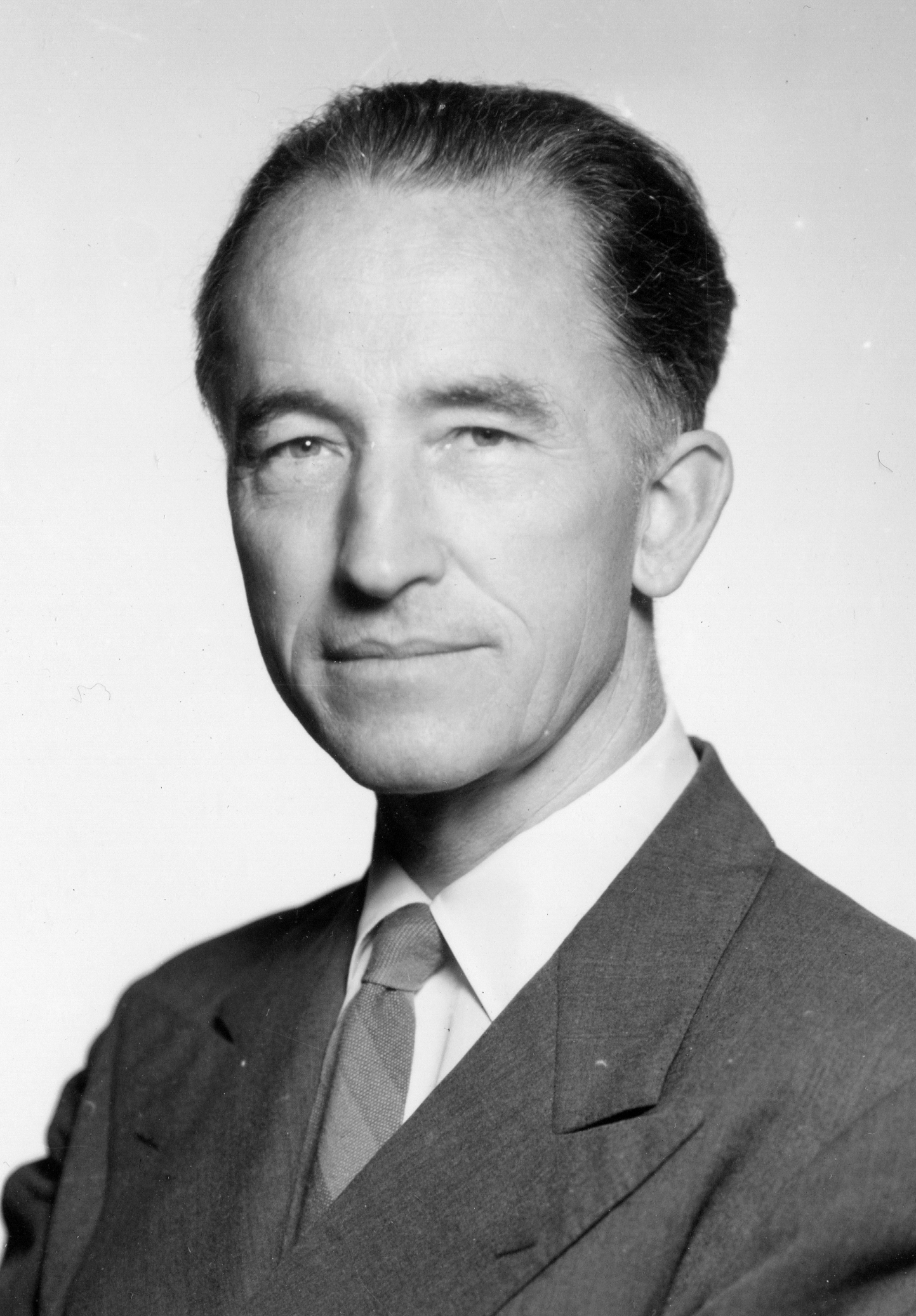
Jacob Bjerknes, forty-two years old, was the oldest son of Vilhelm Bjerknes. His father had founded the Bergen Geophysical Institute in 1917 and had, with Jacob and a handful of Norwegian students, built there the system of ideas – cyclones, warm fronts, cold fronts, occlusions, the polar front – that is still, in 2026, the descriptive vocabulary every television meteorologist uses. In the summer of 1939, Jacob had taken his wife Hedvig Borthen Bjerknes, his eight-year-old son Vil, and his five-year-old daughter Kirsten on what they all believed was an eight-month American lecture tour.1 He was at the University of California, Los Angeles, in April 1940 when the news of the invasion arrived. He had a return ticket. He did not use it.
That decision, taken in a California hotel room in early April 1940, set the trajectory of the next thirty-five years. He founded, at UCLA, the first American department of meteorology at a civilian university. He trained, during the war, over a thousand American military forecasters. He supervised, in 1949, the doctoral thesis of Yale Mintz – the man who would later recruit Akio Arakawa to UCLA and build, with him, the West Coast’s general circulation model. He watched three of his closest oceanographic mentors die in the same year, 1957, and at age sixty responded to their deaths by starting a new line of research on the tropical Pacific. And in two short papers published three years apart, in 1966 and 1969, he identified a feedback mechanism that is now called by his name – the Bjerknes feedback – and that constitutes, to this day, the theoretical core of every numerical model of the most important mode of natural climate variability on the planet.
This is the story of those thirty-five years.
The Bergen Inheritance
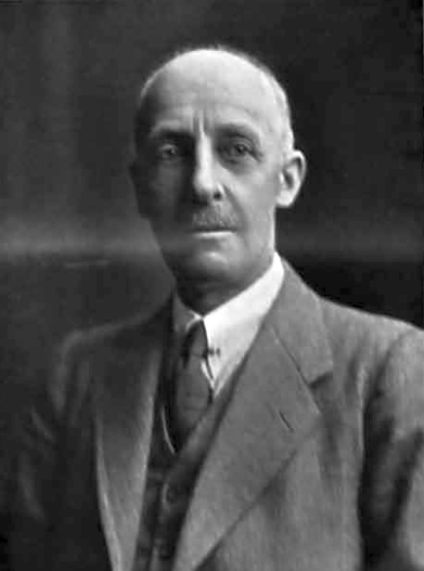
Jacob Aall Bonnevie Bjerknes was born in Stockholm on November 2, 1897.2 His father, Vilhelm Bjerknes, was then a professor of applied mechanics and mathematical physics at the University of Stockholm. The family followed Vilhelm’s career across Europe: to Kristiania (now Oslo) in 1907, to Leipzig in 1913 when Vilhelm accepted the chair of geophysics and the directorship of the new Geophysical Institute there, and finally to Bergen in 1917 when he returned to Norway to found the Geophysical Institute that would become the cradle of modern synoptic meteorology.
The move to Bergen coincided with what is, in the history of the field, the Bergen School’s great decade. Vilhelm, Jacob, Halvor Solberg, Tor Bergeron, Carl-Gustaf Rossby, Erik Palmen, and Sverre Petterssen built, between 1917 and the late 1920s, the entire modern conception of the extratropical cyclone. Jacob’s own 1919 paper “On the Structure of Moving Cyclones,” written when he was twenty-one, introduced the concept of the warm and cold fronts and the frontal cyclone model. The whole Bergen apparatus is already described, with proper footnotes and cross-links, in the Bergen School trilogy of this blog, so I will not re-walk that ground here. What matters for this story is that Jacob entered the 1930s as the heir of the most important meteorological research tradition of the twentieth century, and that he spent the decade running it from a practical base: as director of the Bergen Weather Bureau from 1931 onwards, and as the Bergen Geophysical Institute’s de facto operational arm while Vilhelm grew older.
He had, by his late thirties, a reputation as the Bergen School’s most capable practical meteorologist. What he did not yet have was a theoretical signature of his own – an idea, separable from his father’s, that would be called by his name alone. That would come later. First there was the war.
Eight Months in California
In the summer of 1939 the American Geophysical Union and a consortium of American universities invited Jacob Bjerknes to an eight-month American lecture tour. The plan was straightforward. The family would sail from Bergen in July, spend a few weeks settling in Washington DC, travel by train across the United States visiting Chicago, Wisconsin, the University of California Berkeley, and Los Angeles, and return to Norway in early 1940 in time for Jacob to resume his duties at the Bergen Weather Bureau. Hedvig – the daughter of a Bergen ophthalmologist – packed for an American spring. Vil, aged eight, was taken out of school on the understanding that he would return in February or March.
Germany attacked Poland on September 1, 1939, while the Bjerknes family was on the train crossing the American Midwest. The United Kingdom and France declared war on September 3. Norway, like Sweden and Denmark, declared neutrality. The lecture tour continued. Jacob reached UCLA in late autumn. He was still giving lectures on the Bergen School’s polar-front theory to American audiences when, on April 9, 1940, the Wehrmacht crossed the Norwegian border.
The decision to stay in America was not the family’s alone. It was, in the narration Hedvig later gave to Arnt Eliassen for the 1995 National Academy biographical memoir, a family decision made over the course of several weeks during which the news from Norway was uniformly bad.3 Jacob’s American hosts at UCLA offered him a permanent faculty appointment if he wanted it. Other offers came from Chicago, where Carl-Gustaf Rossby had become a dominant figure, and from MIT. Jacob chose UCLA. Hedvig’s explanation to Eliassen of that choice is one of the most remarkable details of the whole story, because it anticipates, by a quarter century, the scientific problem Jacob would spend his last decade solving: he chose Los Angeles, she said, because it was close to the Scripps Institution of Oceanography at La Jolla. He believed that meteorologists and oceanographers should work together, and he wanted to be near the oceanographers.4
It is the kind of remark that acquires its meaning only in retrospect. In 1940, nobody was publishing seriously on how the atmosphere and the ocean interact. The fields were institutionally separate: meteorology at the universities and national weather services, oceanography at Scripps and Woods Hole. Atmospheric scientists thought of the ocean as a slow, warm boundary condition. Oceanographers thought of the atmosphere as a prescribed wind stress. Jacob Bjerknes, in April 1940, in a Los Angeles hotel room, deciding where to spend the rest of his career, bet on a field that did not yet exist. He did it, Hedvig said, because he believed it would eventually matter.
The offer he accepted was for the founding chair of the University of California Los Angeles Department of Meteorology, a new unit the university had decided to create partly in anticipation of America’s entry into the war. Jacob took it in 1940. He was forty-three years old. He had a wife, two children, an accented English, no clear sense of when or whether he would see Norway again, and a faculty salary denominated in US dollars. Vilhelm, who was seventy-eight and in failing health, was in Oslo under German occupation. Jacob could not have known it, but he would see his father only once more: in 1947, for a brief visit after the war. Vilhelm would die in Oslo in April 1951, eleven years to the day after the German invasion.5
The Department
The UCLA Meteorology Department that Jacob Bjerknes founded in 1940 was, for its first three years, almost entirely in the business of training American military forecasters.6 America entered the war in December 1941. The Army Air Corps and the Navy both needed large numbers of weather officers for aircraft operations, for amphibious landings, for the entire global war the United States was about to fight. UCLA was one of the handful of American institutions that could provide the training. Jacob ran the program. Over the course of the war he personally trained or supervised the training of more than a thousand American meteorologists – a figure that does not sound enormous until you realise that the entire pre-war American meteorological profession was about the same size. The postwar generation of American civilian and military forecasters was, to a substantial degree, a Bjerknes generation.
His faculty colleagues in those early UCLA years included, almost immediately, a second Norwegian: Jorgen Holmboe, who also found himself in California when Norway was invaded and who also stayed. Holmboe and Bjerknes co-authored several papers in the 1940s on the dynamics of the atmosphere’s general circulation; Holmboe’s 1945 paper on baroclinic instability (known to every graduate student as the Eady-Holmboe analysis) was one of the foundational works of mid-latitude dynamical meteorology. Morris Neiburger joined the department in 1941 and would remain there for half a century, developing the study of marine stratocumulus clouds off the California coast and eventually becoming one of the founders of American air-pollution meteorology. James London arrived in the late 1940s. Zdenek Sekera came in 1949. By the end of the decade UCLA had, along with MIT and Chicago, one of the three leading meteorology departments in the United States.
One of the first students Jacob supervised was Jerome Namias, who would go on to found the long-range forecasting program at the U.S. Weather Bureau and at Scripps. Another, arriving in the mid-1940s, was a Manhattan-born humanist with a Columbia master’s degree in geology and a latter-career switch into meteorology: Yale Mintz. Mintz defended his PhD under Jacob in 1949. It was the second doctorate the UCLA Meteorology Department ever awarded. Mintz stayed on the faculty. Twelve years later, after a stretch of descriptive climatology under Bjerknes’s general-circulation project, he would read Phillips’s 1956 experiment, decide UCLA needed its own general circulation model, and recruit Akio Arakawa from the Japan Meteorological Agency. The UCLA GCM I wrote about on Tuesday is, in institutional lineage, a Bjerknes program. Jacob did not write a line of the code. He had, however, hired every single one of the people who did.
1951
On April 9, 1951 – exactly eleven years to the day after the German invasion of Norway – Vilhelm Bjerknes died in Oslo. He was eighty-eight. He had spent the war under German occupation, had survived it, and had resumed, in his last years, a fragmentary correspondence with his son. The two had been able to see each other exactly once in the eleven years since they had last been in the same room: during Jacob’s 1947 visit to Norway. Jacob did not attend the funeral. International travel in April 1951 was still slow and expensive, and the Bjerknes family in Los Angeles had reasons of their own not to make the trip.7
Jacob’s reaction, as far as I can reconstruct it from the limited primary sources, was to throw himself more deeply into the American scientific community. He had become, in 1945, the first recipient of the AGU’s William Bowie Medal who was not himself American by birth. He would, through the 1950s, collect most of the rest of the honours an active meteorologist could receive: the Losey Atmospheric Sciences Award in 1963, the Carl-Gustaf Rossby Research Medal in 1960 (the AMS’s highest award, named after his father’s Bergen student), the International Meteorological Organization Prize in 1959, and in 1966 the National Medal of Science from Lyndon Johnson. He served as president of the International Union of Geodesy and Geophysics from 1948 to 1951 and of the American Meteorological Society in 1959. By the end of the 1950s he was, according to the obituary written by Arnt Eliassen, the most honoured meteorologist alive.8
His science in the 1950s was, by his own standards, less original than the Bergen-School years. He worked on the general circulation problem, on the heat balance of the atmosphere, on the influence of sea-surface temperatures in the Atlantic on European weather patterns. The Atlantic work, which began in 1959 with a paper on “Atlantic air-sea interaction,” was the first sustained piece of what would later be called air-sea coupling theory. It drew on data from a hemisphere Jacob could only see in retrospect across a continent and an ocean he would never again live on. By 1960 he was sixty-two years old, thirteen years into his UCLA tenure, a decade past his father’s death, and looking, by most measures of an academic career, like a man settling into a distinguished emeritus phase.
The Three Deaths of 1957
Then came the year 1957.
Three men died that year who, together, had been Jacob Bjerknes’s closest scientific mentors outside his immediate family. Carl-Gustaf Rossby, Norwegian-American, student of Vilhelm’s in Bergen in the 1920s, founder of the meteorology programs at MIT and the University of Chicago, and arguably the single most important meteorologist of the interwar and wartime generation, died suddenly in Stockholm on August 19, 1957, at sixty-eight. Harald Ulrik Sverdrup, Norwegian oceanographer, discoverer of the Sverdrup transport and the canonical textbook on the oceans, had died in Oslo on August 21, 1957, two days after Rossby. Bjorn Helland-Hansen, Norwegian oceanographer of the previous generation and a close collaborator of Vilhelm’s in the 1910s and 1920s, had died earlier in the year, on April 22, 1957, at eighty.9
Three Norwegians in the ocean-atmosphere tradition, dead within four months of each other, in the same year the International Geophysical Year was scheduled to begin.
Jacob Bjerknes was sixty years old in August 1957. The Bergen generation that had shaped him was now, with his father’s death six years earlier, almost entirely gone. The IGY, which would run from July 1957 to December 1958, was about to collect, through an internationally coordinated network of research ships, island weather stations, radiosondes, and early weather satellites, the most complete set of observations of the global atmosphere and ocean ever assembled. Much of the instrumentation was being deployed across the tropical Pacific, a region that had, until then, been observationally nearly opaque to meteorology. And the IGY would, as it happened, coincide with one of the strongest El Niño events in the instrumental record.
The Bjerknes who began to read the IGY data in the late 1950s was not, any longer, a Bergen-School synoptic meteorologist working on European cyclones. He was a coupled-systems climate dynamicist, thirty years before anyone else understood what that phrase meant. It is very unusual for a scientist to switch research programs in his sixties. What Jacob did was more than a switch. It was a reinvention.
What Gilbert Walker Had Found
To understand what Bjerknes did in the late 1960s, you have to understand what Gilbert Walker had done forty years earlier.
Sir Gilbert Thomas Walker (1868-1958) was a Cambridge-trained mathematician who had been appointed Director General of Observatories in India in 1904, at the peak of the British Raj.10 His assignment was to predict the Indian summer monsoon. Failure of the monsoon meant famine; Walker’s employer, the Government of India, was acutely interested in any statistical regularity that might give advance warning of a bad year. Walker, who had no particular background in meteorology but had an enormous aptitude for statistics, responded by putting his staff of Indian clerks to work computing, by hand, thousands of lagged correlations between pressure, temperature, rainfall, and winds at every weather station in the global observing network.
The work was massive. Walker’s 1923 paper “Correlation in seasonal variations of weather, VIII: A Preliminary Study of World Weather” reports correlations computed from decades of records at dozens of stations.11 The correlations were computed by hand, by clerks, with mechanical calculators and in some cases with pencil and paper, over a period of years. The Pune weather office’s staff in the 1910s and 1920s included, at Walker’s instigation, a permanent team of human calculators whose only job was to grind out thousands of lagged correlation coefficients between pressure series at every weather station in the British Empire. If you wanted to know whether winter pressure at Madeira was correlated with the next summer’s Indian monsoon rainfall at a six-month lag, Walker’s clerks could tell you. The volume of the computation is one of the hidden scandals of imperial meteorology: a major scientific discovery rests on the uncredited labour of dozens of Indian clerks who performed, for decades, what a 2026 laptop would do in under a second.
To handle the statistics properly Walker had to work out, in the 1920s, the mathematics of autoregressive time series – the equations now known as the Yule-Walker equations, named jointly after Walker and the British statistician Udny Yule. He did this as a side effect of wanting to know whether the Indian monsoon would fail. Very few scientific careers in any field have generated this kind of mathematical infrastructure as collateral damage.
The patterns Walker found were striking. He identified what he called the North Atlantic Oscillation, a pressure see-saw between Iceland and the Azores that is now one of the dominant patterns of European winter climate variability. He identified what he called the North Pacific Oscillation, a similar see-saw in the North Pacific. And, most importantly for the story I am telling here, he identified what he called the Southern Oscillation: a pressure see-saw between Darwin in northern Australia and Tahiti in the central South Pacific, with a period of something like three to seven years. When Darwin pressure was high, Tahiti pressure was low. When Darwin was low, Tahiti was high. The two oscillated together, out of phase, on a multi-year time scale.
Walker had no idea what the Southern Oscillation was. He had, by statistical methods alone, identified a pattern. He had no mechanism to explain why it existed, and he was dismissed by most of the meteorological community of his time as a statistical empiricist without a physical theory. He retired from India in 1924, moved to Imperial College London, continued to publish quietly for another decade, and died in November 1958 at the age of ninety, without having seen his discovery either mechanistically explained or broadly accepted.12
He died, to put it exactly, seventeen months after the International Geophysical Year began collecting the data that would vindicate him – and eleven years before Jacob Bjerknes, in Los Angeles, published the paper that would do the explaining.
The 1957-58 El Niño
The International Geophysical Year’s observational effort across the tropical Pacific was, in scale, without precedent. Research ships sailed hundreds of thousands of miles taking oceanographic measurements. Island weather stations on Christmas Island, Canton Island, Easter Island, and the Galapagos collected hourly surface data. The first weather satellite was still three years away, but radiosondes went up from dozens of IGY stations every twelve hours. What the data showed, in the months between July 1957 and December 1958, was a tropical Pacific very different from its normal state. The trade winds along the equator had weakened. The normally cold cold-tongue of surface water along the Peruvian coast had been replaced by a mass of warm water extending west across the basin. The Peruvian anchoveta fishery, in those months, collapsed. The South American fishmeal industry, which supplied global animal feed, took a hit that was felt in Chicago commodity markets.
The IGY had captured, in unprecedented scientific detail, what Peruvian fishermen had known about for centuries: el nino, the warm southward current that arrives around Christmas and kills the anchoveta catch. What the fishermen had not known, and what Walker’s statistical work had only hinted at, was that this Peruvian coastal event was connected to simultaneous changes in air pressure at Darwin and Tahiti, to weakened trade winds, and to weather anomalies as far away as North America.
The person who, in the late 1950s and early 1960s, began to piece this together from IGY data was the German-American oceanographer Klaus Wyrtki, who had settled at Scripps and then at the University of Hawaii.13 Wyrtki’s 1961 monograph on the physical oceanography of the equatorial Pacific laid out the basin-scale picture. Jacob Bjerknes read Wyrtki. He read the pressure data Walker had collected. He read the SST data the IGY had produced. He was, in the early 1960s, in the rare position of knowing the atmospheric side deeply (from his Bergen-School apprenticeship), the Atlantic air-sea-interaction literature (from his own 1950s work), and the IGY Pacific data (from his UCLA proximity to Scripps). He began to put the pieces together.
The 1966 Paper
In 1966 Bjerknes published a short paper in the Swedish journal Tellus titled “A possible response of the atmospheric Hadley circulation to equatorial anomalies of ocean temperature.”14 It is nine pages long. Its argument, compressed to a single sentence, is that the atmosphere’s tropical overturning circulation (the Hadley cell) responds to sea-surface temperature anomalies in the equatorial Pacific – rather than, as was generally assumed at the time, being driven entirely by solar forcing and independent of ocean temperature.
The paper is cautious. It is titled “A possible response.” The argument is qualitative rather than quantitative. Bjerknes does not claim to have found a coupled mode of atmosphere-ocean variability; he claims only to have shown that ocean temperatures could, in principle, drive changes in the Hadley circulation. Read in isolation, the 1966 paper looks like a modest contribution to tropical-atmospheric dynamics. Read in light of what came next, it is clearly a rehearsal.
The 1969 Paper
Three years later, in the March 1969 issue of the Monthly Weather Review, Bjerknes published a paper titled “Atmospheric teleconnections from the equatorial Pacific.”15 It is ten pages long. It is one of the most important papers in the history of climate science.
The paper does five things, interleaved across its ten pages. It unifies Walker’s Southern Oscillation – the Darwin-Tahiti pressure see-saw – with the Peruvian El Niño – the warm-water events – as two manifestations of a single coupled system. It names the zonal atmospheric circulation that runs from Indonesia (rising air) across the Pacific to Peru (sinking air) the Walker circulation, in a deliberate tribute to the British mathematician who had identified its statistical fingerprint forty years earlier. It identifies the Bjerknes feedback – the positive feedback between trade winds, upwelling, sea-surface temperature, and atmospheric pressure that maintains both the normal cold-tongue / warm-pool pattern of the Pacific and the inverted warm-east / weak-trades pattern of El Niño. It shows that North American weather anomalies during the 1957-58 El Niño were part of this system – the first explicit formulation of tropical-extratropical teleconnections. And it anticipates, in a way nobody would have credited at the time, the entire field of climate dynamics as it would develop over the next fifty years.
The feedback can be described in three sentences without any equations. In the normal state of the tropical Pacific, strong easterly trade winds drag surface water westward, pile up a warm pool over Indonesia, and expose cold deep water along the Peruvian coast. The east-west temperature contrast drives the atmospheric Walker circulation, with rising air over the warm west and sinking air over the cold east, which in turn maintains the trade winds. Weaken the trade winds even slightly, and the warm pool slides east, warming the eastern Pacific, weakening the Walker circulation, and weakening the trade winds further – the positive feedback that Bjerknes recognized, and that every modern model of El Niño is built around.16
Bjerknes’s own wording, in the 1969 paper, is more careful and less algorithmic than my paraphrase. He describes the phenomenon as a “chain reaction” in which “an intensifying Walker Circulation also provides for an increase of upwelling of cold water off South America,” and by the inverse reasoning, a weakening of the Walker circulation reduces upwelling, warms the eastern Pacific, and further weakens the circulation.17 It is a sentence the 1920s Walker would have understood instantly if he had lived to read it. He had correlated the pattern statistically in the 1920s. He had died, in 1958, without knowing the mechanism. Bjerknes, in 1969, gave it to him.
The Schematic

Bjerknes did not draw that schematic – the version reproduced above is a modern illustration from Wikimedia Commons, with German labels, of the structure Bjerknes described. Compressed to its minimum, the diagram says the following:
Upper panel (normal conditions): Easterly trade winds blow along the equator from Peru toward Indonesia. They drag warm surface water westward, building a warm pool over the western Pacific. Below that warm pool, the thermocline – the sharp boundary between warm surface water and cold deep water – is deep, at 150 to 200 metres. Above the pool, the warm ocean heats and moistens the overlying atmosphere, which rises as convection, producing the heavy tropical rainfall that characterizes the Indonesian maritime continent. The rising air, moving east aloft, descends over the eastern Pacific – where cold upwelled water, by contrast, cools and dries the atmosphere above, producing the dry coastal-desert climate of Peru and Chile. The zonal atmospheric circulation rising in the west and sinking in the east is the Walker circulation.
Lower panel (El Nino): The trade winds weaken. The accumulated warm pool, no longer held in place by strong trades, flows eastward along the equator as a train of oceanic Kelvin waves. The thermocline in the east rises, suppresses upwelling of cold water, and warms the surface of the eastern Pacific by several degrees. The atmospheric convection that normally sits over Indonesia shifts east along with the warm water. The Walker circulation, deprived of its west-east temperature contrast, weakens or even reverses. The eastern Pacific’s cold tongue disappears; the Peruvian anchoveta fishery collapses; North American storm tracks shift; droughts and floods occur from Australia to Brazil.
The two states are not independent events. They are two phases of a single oscillation, driven by the slow dynamics of the equatorial ocean, coupled to the atmosphere through the feedback Bjerknes identified. The oscillation itself – the ENSO cycle – has a period of roughly two to seven years, set by the slow return of oceanic Rossby waves from the western boundary of the Pacific basin. But the central idea, the thing that makes ENSO a self-sustaining climate mode rather than a random fluctuation, is the Bjerknes feedback.
The 1969 paper contains no equations describing the feedback rigorously. It is a qualitative argument. The mathematical development would come later, from Klaus Wyrtki at Hawaii (1975), from Mark Cane and Stephen Zebiak at Lamont-Doherty (1985), from the Schopf-Suarez delayed-oscillator theory (1988), and from Fei-Fei Jin’s recharge-oscillator theory (1997). Each of these later contributions is a mathematical formalization of what Bjerknes had described in 1969 in a chain of physical reasoning, two paragraphs long.
The Reception
The 1969 paper did not produce an immediate revolution. It was cited, in the first few years after publication, by a small group of specialists – Wyrtki, Namias, Jerome Namias’s Scripps colleagues, a handful of tropical meteorologists at NCAR. The American National Meteorological Center did not, through the 1970s, operationally forecast El Niño events. There was no ENSO community as such. Climate dynamics, as a research field with journals and conferences and tenure cases, did not yet exist.
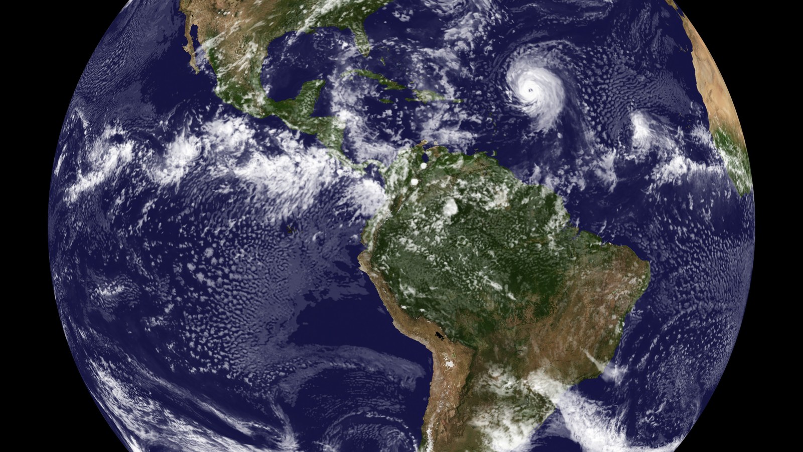
What produced the revolution was the 1972-73 El Niño event. It was observed in real time, for the first time, using the framework Bjerknes had provided. The trade winds had weakened in the spring of 1972; the warm pool had slid east; the Peruvian anchoveta fishery collapsed in the autumn and winter; fishmeal prices tripled; Chicago soybean futures doubled as markets scrambled for an alternative animal feed. The event made the cover of Time. It made Bjerknes’s 1969 paper, retrospectively, urgent.
By 1975, the tropical-Pacific research community had expanded from perhaps a dozen scientists worldwide to several hundred. The Wyrtki 1975 paper on the dynamical response of the equatorial Pacific to atmospheric forcing set out the wave dynamics that Bjerknes had only hinted at.18 In 1985 Mark Cane and Stephen Zebiak at Columbia’s Lamont-Doherty Earth Observatory completed the first coupled atmosphere-ocean model of ENSO, the Cane-Zebiak model, which in 1986 produced the first successful prospective forecast of an El Niño event (the 1986-87 warming) from a numerical simulation.19 The forecast was published in Nature in June 1986. It was the first successful numerical coupled-system forecast in climate science.
The 1982-83 El Niño – the largest of the instrumental record at the time – did almost eight billion dollars’ worth of damage globally and was the event that made the word “El Niño” part of the public vocabulary. It also exposed, spectacularly, the limits of the 1980s observational system.
On March 28 and April 4, 1982, the Mexican volcano El Chichon erupted, injecting a substantial load of sulphate aerosol into the lower stratosphere. The aerosol formed a veil that, over the following months, drifted westward around the Earth and sat over the tropical Pacific for most of 1982. Satellite radiometers that measure sea-surface temperature from space look through the stratosphere to do so, and the El Chichon aerosol scattered the infrared signal in a way that made the tropical Pacific SSTs appear, to a casual operational forecaster, approximately normal. The actual ocean beneath the aerosol was warming, in real time, into one of the largest El Niño events in the instrumental record. The satellite data said there was no event. The aerosol said there was no event. The surface moorings, which had been installed only sporadically, were not yet dense enough to contradict the satellite. By the time operational forecasters in the American and Peruvian weather services had worked out, through the autumn of 1982, that they were inside a record-breaking event, the peak had already passed. Fisheries had collapsed; rainfall in Peru and Ecuador was three to five times normal; Pacific cyclones had struck Tahiti; Australian rainfall had collapsed. Nobody had predicted it. Nobody had even recognised it while it was happening.
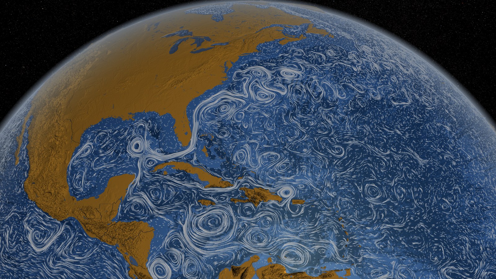
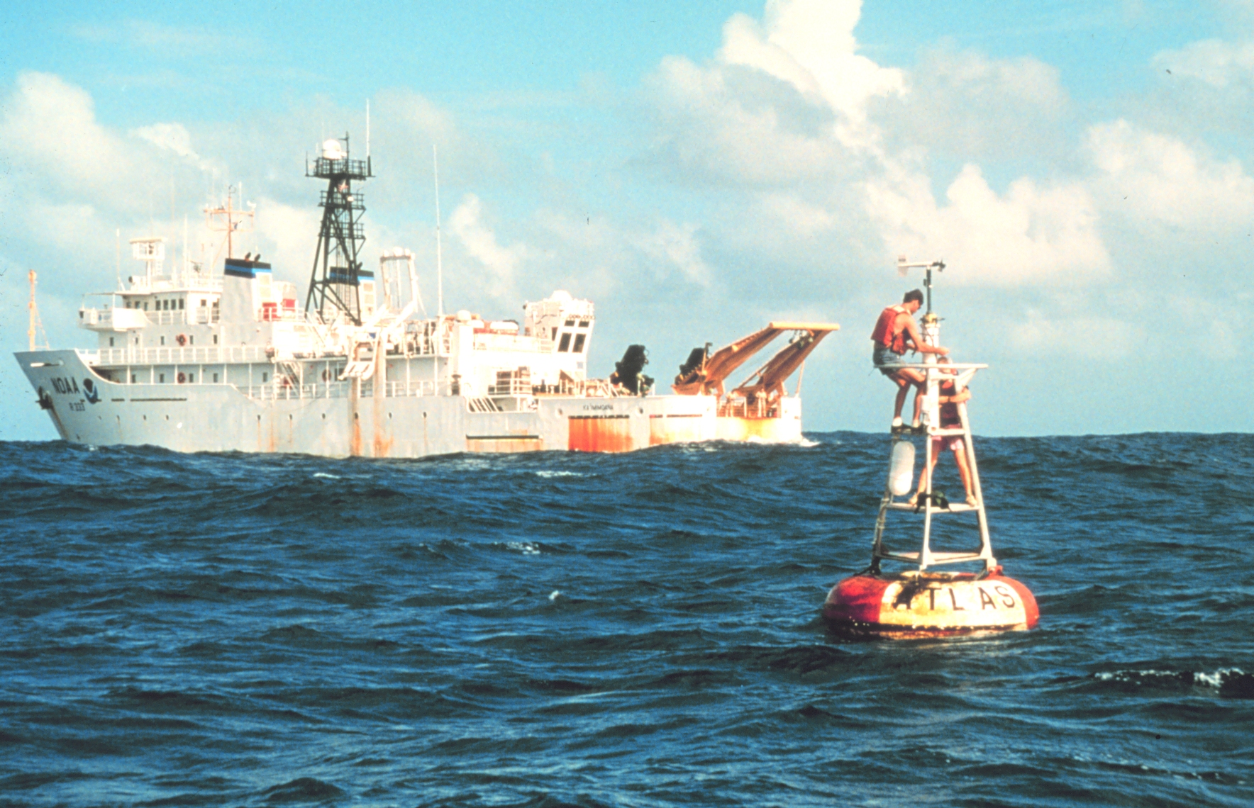
The professional humiliation was substantial. The response was institutional. Between 1985 and 1994 an international research program called the Tropical Ocean-Global Atmosphere program, TOGA, deployed a permanent set of approximately seventy deep-water moorings across the equatorial Pacific. Each mooring measured, every hour, subsurface ocean temperature and current from the surface down to 500 metres, and surface meteorological variables (wind, air temperature, humidity). The data streamed in real time to shore stations and onward to weather centres. By the end of TOGA the tropical Pacific was the single best-observed region of the ocean on Earth. Every modern operational ENSO forecast – the 6- to 9-month lead predictions now issued routinely by NOAA’s Climate Prediction Center, by ECMWF’s SEAS5 system, by the European Copernicus Climate Change Service – depends on the data those moorings continue to collect in 2026. The array is called TAO/TRITON: Tropical Atmosphere-Ocean, maintained jointly by NOAA and the Japan Agency for Marine-Earth Science and Technology. Its construction is a direct response to the failure of 1982. Its theoretical framework – the reason anyone knew that placing moorings across the equatorial Pacific would pay off scientifically – was the framework Bjerknes had published thirteen years earlier.
All of this was, from Bjerknes’s point of view, a slow vindication. He retired from UCLA in 1965, the year before his 1966 Tellus paper, and took emeritus status. He lived to see the 1972-73 event, which was the proof his framework had been waiting for. He did not live to see the Cane-Zebiak model or the TOGA program. He died in Los Angeles on July 7, 1975, age seventy-seven.20
The Machines That Proved Him Right
Bjerknes himself did not use computers for the 1966 or 1969 papers. The synthesis was done with pencil, paper, IGY observational tables, and the kind of cross-correlation reasoning that Walker had done by hand forty years earlier. What came next – the quantitative, predictive, operational theory of ENSO that turned Bjerknes’s 1969 framework into a tool for forecasting El Nino events months in advance – was computational from beginning to end. The people who did the computing used a succession of machines, each of which imposed its own algorithmic constraints on what the science could express.
The first of these machines were the ones already running at Lamont-Doherty Earth Observatory in the mid-1980s. Mark Cane had come to Lamont in 1981 from MIT, where he had worked with Jule Charney on tropical dynamics. Stephen Zebiak was then his postdoc. The machine they had access to was a DEC VAX 11/780, a minicomputer running the VMS operating system at about 1 million instructions per second, with a few megabytes of real memory and a disk-based virtual memory system that let them pretend, for most workloads, that they had more.21 A VAX 11/780 was roughly two orders of magnitude slower than the 1984-vintage Cray X-MP that Syukuro Manabe and Kirk Bryan were by then using at GFDL, and three orders of magnitude slower than any 2026 laptop. What it was, though, was genuinely available: a university research group could sign up for time and get it, rather than negotiating weekend slots on a shared national laboratory machine.
What Cane and Zebiak did in 1985 was to build, on the VAX, a new kind of climate model. The full coupled atmosphere-ocean general circulation model – Manabe and Bryan’s 1969 system, or its 1985 descendant running on GFDL’s Cray – was, in the mid-1980s, too expensive for a university group to use for ENSO forecast experiments. A single twelve-month coupled forecast, on a full GCM, could take months of machine time. The Cane-Zebiak model was an intermediate-complexity model: a compromise between the full nonlinear GCM and the purely analytical theoretical models that Wyrtki and others had been developing in the 1970s.
The model’s architectural choices are worth enumerating because they are the canonical example of algorithmic restraint in climate science. The ocean component was a linearised shallow-water model of the equatorial Pacific, with a single active baroclinic mode and a simplified mixed-layer surface heat budget. The atmosphere component was a linearised steady-state model of tropical circulation – a so-called Gill atmosphere, after Adrian Gill’s 1980 paper on equatorial heating22 – in which the wind response to a tropical heating anomaly could be computed as a linear operator acting on the SST field. The two components exchanged wind stress (atmosphere to ocean) and surface heat flux / SST feedback (ocean to atmosphere) at each time step. The coupling expressed the Bjerknes feedback explicitly: warm eastern-Pacific SST drove weaker trade winds, weaker trade winds drove warmer eastern SST, all in one compact linear system. The model had no resolved synoptic weather. It had no atmospheric Rossby waves outside the tropics. It had no thermohaline circulation in the ocean. It could not simulate clouds, precipitation, or any extratropical weather at all. What it could do was produce the equatorial Pacific’s coupled mode, cheaply, and integrate it for decades of simulated time on a VAX that belonged to a university research group.
The 1986 Nature paper in which Cane, Zebiak, and Sean Dolan reported their first prospective forecast of the 1986-87 El Nino using this model is, if you care about the history of numerical climate modelling, a landmark.23 It was the first time a coupled atmosphere-ocean system had been successfully forecast, from observations, ahead of a verifiable event. The entire field of seasonal-to-interannual climate prediction – which is now a routine operational enterprise at every major weather centre in the world – dates from that paper. And the machine behind the paper was not a supercomputer. It was the kind of departmental minicomputer that, in 2026, would be a recycling fee at a university surplus sale.
The Cane-Zebiak model’s algorithmic simplicity was its scientific strength. Because the model was linear in structure, its dynamics could be analysed mathematically. The delayed-oscillator theory of ENSO, published by Peter Schopf and Max Suarez at NASA Goddard in 1988, is essentially an analytical explanation of why the Cane-Zebiak model oscillates: warm SST anomalies in the eastern Pacific generate westward-propagating oceanic Rossby waves, which reflect off the western boundary as eastward-propagating Kelvin waves, which return to the eastern Pacific months later with the opposite sign, flipping the state of the coupled system.24 The oscillation period emerges from the basin-crossing times of these waves. This is the theoretical architecture that underpins every modern ENSO forecast. It was derivable, and testable, because Cane and Zebiak had chosen to build a model simple enough to analyse.
Subsequent ENSO modelling moved in two directions at once. The theoretical side, in the 1990s and 2000s, refined the delayed-oscillator picture into the more complete recharge-oscillator theory of Fei-Fei Jin in 1997, which treated the equatorial Pacific ocean’s heat content as a slowly varying state variable that recharges during La Nina and discharges during El Nino.25 The operational side moved, by the late 1990s, onto full coupled general circulation models running on vector supercomputers: the NCEP Coupled Forecast System version 1 (CFSv1, 2004) and its successor CFSv2 (operational since 2011), the ECMWF System 4 (2011) and SEAS5 (2017), the UK Met Office GloSea series, and the Tokyo Climate Center’s JMA coupled system. These are all full GCMs with atmosphere grids at roughly 50 km horizontal resolution, ocean grids at 25 to 50 km, and ensemble members run in parallel on HPE Cray and NVIDIA GPU-enabled supercomputers. The Fortran I wrote about in the Fortran series is the language all of them run on. The Bryan-Cox / NEMO / MOM6 ocean code I wrote about yesterday is the ocean component all of them use.
The data that feeds them is the data Bjerknes did not have. Roughly seventy TAO/TRITON buoys, moored along the equator from 8 degrees north to 8 degrees south and spanning from 137 degrees east (west of Papua New Guinea) to 95 degrees west (off Peru), measure subsurface ocean temperature from the surface down to 500 metres, surface air temperature, humidity, wind, pressure, and (at a subset of locations) shortwave radiation, every ten minutes, and transmit the data by satellite to the Pacific Marine Environmental Laboratory in Seattle. The TAO array was proposed in 1984 by Stan Hayes at PMEL and Larry McPhaden (who would later lead the operation for three decades) as a direct response to the 1982-83 satellite failure I described above.26 It was built out through TOGA (1985-1994), handed to routine operational maintenance in 1995, and has been producing continuous data ever since. As of 2026 it is supplemented by the Argo array of roughly 4 000 autonomous profiling floats in the world’s oceans, which surface every ten days to transmit temperature and salinity profiles. Between them, TAO and Argo give 2026’s forecasters something Bjerknes could only have dreamed of: a continuous real-time picture of the upper-ocean state that the theoretical framework of the 1969 paper tells them exactly how to interpret.
The forecast skill, as of 2026, is what it is. Operational ENSO forecasts from NOAA’s Climate Prediction Center are skilful at lead times of roughly six to nine months for the dominant ENSO indices (the Nino 3.4 SST anomaly). They are less skilful when the coupled system is transitioning between states; they were, in particular, publicly embarrassed in early 2024 when most operational systems over-forecast a transition to La Nina conditions that did not materialize as quickly as predicted. The so-called spring barrier – the tendency of ENSO forecast skill to degrade rapidly for forecasts initialized in March and April – is an unsolved problem, one of the few that remains. But for late-summer-through-winter forecasts of the following winter’s state, the skill is genuine and substantial, and every industry from California agriculture to Peruvian fisheries to Australian wheat markets now makes plans that depend on it.
All of this – the VAX of 1985, the TAO deployments of the late 1980s, the Cray-based CFSv2 of 2011, the HPE Cray systems of 2026 – rests on a four-paragraph argument in the Monthly Weather Review of March 1969. Bjerknes did not live to see any of the computational machinery that proved him right. He did the science with a pencil. Three generations of scientists since have used computers to demonstrate, with quantitative rigour, that the pencil was right.
The Family Arc
There is one more way to tell this story, which is that it is a story about a father and a son. Vilhelm Bjerknes, born in 1862, founded the science of synoptic meteorology in Bergen between 1917 and 1930. His son, born thirty-five years later, founded the science of climate dynamics in Los Angeles between 1940 and 1969. The two founders, father and son, between them defined twentieth-century atmospheric science. The family tradition was the idea that the weather is a continuous fluid mechanics problem; the family’s particular genius was the ability to translate that abstract idea into specific, testable, communicable scientific programs. Vilhelm’s program was the extratropical cyclone. Jacob’s program was the coupled tropical system. They sit together in the history of the field as perhaps its two most consequential programmatic statements.
Jacob was sixteen years old when his father took the chair at Leipzig in 1913 and eighteen when the family moved to Bergen in 1917. He was twenty-one when he published “On the Structure of Moving Cyclones” in 1919. He was forty-two when he left Norway in July 1939 on an eight-month lecture tour, and forty-three when he decided in Los Angeles, in April 1940, not to go back. He was fifty-four when Vilhelm died. He was sixty in 1957 when his three Bergen-adjacent oceanographic mentors died. He was sixty-nine when he published the 1966 paper, seventy-one when he published the 1969 paper. He was seventy-seven when he died in Los Angeles on July 7, 1975. His wife Hedvig outlived him by twenty-three years; she died in 1998. His son Vil, who had been eight years old when the family’s eight-month lecture tour began in 1939, became an American citizen, married, had children of his own, and survived his father. His daughter Kirsten, who had been five, did the same.
The family came to California in 1939 and never went home. What they left behind, when the last of them died, was a department at UCLA that had trained a thousand American wartime forecasters and graduated four generations of PhD students, a collection of medals and honours spanning forty years of Scandinavian and American science, and – tucked quietly inside a ten-page paper in the March 1969 issue of Monthly Weather Review – the theoretical skeleton of every climate model that now projects, to the limits of mid-century predictability, what the coupled atmosphere-ocean system of the Earth will do to its temperature, its rainfall, its storms, and its fisheries through the twenty-first century.
The Pacific told him. He listened.
Footnotes
References
Primary sources:
- Bjerknes, J. (1919). “On the Structure of Moving Cyclones.” Geofysiske Publikasjoner 1(2), Oslo.
- Bjerknes, J. (1966). “A possible response of the atmospheric Hadley circulation to equatorial anomalies of ocean temperature.” Tellus 18(4), 820-829. Link.
- Bjerknes, J. (1969). “Atmospheric teleconnections from the equatorial Pacific.” Monthly Weather Review 97(3), 163-172. Link.
- Walker, G. T. (1923). “Correlation in seasonal variations of weather, VIII: A Preliminary Study of World Weather.” Memoirs of the India Meteorological Department 24(4), 75-131.
- Walker, G. T. (1928). “World Weather.” QJRMS 54, 79-87.
- Wyrtki, K. (1975). “El Nino: the dynamic response of the equatorial Pacific Ocean to atmospheric forcing.” J. Phys. Oceanogr. 5(4), 572-584.
- Cane, M. A., Zebiak, S. E., Dolan, S. C. (1986). “Experimental forecasts of El Nino.” Nature 321, 827-832.
Biographical:
- Eliassen, A. (1995). “Jacob Aall Bonnevie Bjerknes, 1897-1975: A Biographical Memoir.” Biographical Memoirs of the NAS 68. PDF.
- UCLA Department of Meteorology (1977). “In Memoriam: Jacob A. B. Bjerknes.” Authors: A. Arakawa, M. Neiburger, M. G. Wurtele. Internet Archive.
- Jacob Bjerknes – Wikipedia.
ENSO science:
- Philander, S. G. H. (1990). El Nino, La Nina, and the Southern Oscillation. Academic Press.
- Wang, C. (2018). “A review of ENSO theories.” National Science Review 5(6), 813-825.
- Jin, F.-F. (1997). “An equatorial ocean recharge paradigm for ENSO. Part I: Conceptual model.” J. Atmos. Sci. 54, 811-829.
- Schopf, P. S., and Suarez, M. J. (1988). “Vacillations in a coupled ocean-atmosphere model.” J. Atmos. Sci. 45, 549-566.
Institutional:
- UCLA Department of Atmospheric and Oceanic Sciences: Department history.
- NOAA Pacific Marine Environmental Laboratory: TAO/TRITON array.
Cross-references in this series:
- The Line That Models Cannot Draw – Vilhelm Bjerknes and the Bergen School; the father.
- Reading the Sky – Bergen School evolution through the 1920s-30s.
- The Ghost in the Grid – front detection in modern models.
- The Swedes Got There First – Rossby and the Swedish postwar modelling program; one of the three deaths of 1957.
- The Fireman and the Visionary – Yale Mintz and Akio Arakawa at UCLA; Mintz was Jacob’s PhD student.
- The Man Who Fit the Entire Ocean in Half a Megabyte – Kirk Bryan and ocean general circulation modelling at GFDL; the coupled-systems work that Bjerknes’s framework made possible.
-
Eliassen, A. (1995). “Jacob Aall Bonnevie Bjerknes, 1897-1975: A Biographical Memoir.” Biographical Memoirs of the National Academy of Sciences 68, 3-20. The eight-month tour and family composition are documented there from Hedvig Bjerknes’s direct testimony to Eliassen. PDF at biographicalmemoirs.org. ↩
-
Eliassen 1995, same reference as footnote 1; also Wikipedia – Jacob Bjerknes. ↩
-
Eliassen 1995, same reference as footnote 1. ↩
-
Eliassen 1995. Hedvig’s testimony about why UCLA is in Eliassen’s biographical memoir; the Scripps-proximity rationale is among the more striking details of the whole narrative. ↩
-
Vilhelm Bjerknes’s death date of April 9, 1951 is confirmed by Wikipedia – Vilhelm Bjerknes and by the National Academy of Sciences biographical memoir of Vilhelm. The coincidence with the April 9, 1940 German invasion date is real. ↩
-
Eliassen 1995, same reference as footnote 1. UCLA Department of Atmospheric and Oceanic Sciences history page at atmos.ucla.edu/history-2 provides additional institutional detail. ↩
-
Eliassen 1995; UCLA Department of Meteorology In Memoriam for Jacob Bjerknes, 1977, authors: A. Arakawa, M. Neiburger, M. G. Wurtele. Internet Archive copy. ↩
-
Eliassen 1995, same reference. Jacob Bjerknes received the William Bowie Medal (AGU, 1945), the Losey Atmospheric Sciences Award (1963), the Rossby Research Medal (AMS, 1960), the IMO Prize (1959), and the National Medal of Science (1966), among many others. He served as IUGG president 1948-1951 and as AMS president in 1959. ↩
-
Deaths verified through individual Wikipedia biographies: Carl-Gustaf Rossby (d. August 19, 1957), Harald Sverdrup (d. August 21, 1957), Bjorn Helland-Hansen (d. April 22, 1957). ↩
-
Gilbert Walker – Wikipedia; Royal Meteorological Society obituary of Walker, Weather 13, 309-311 (1958). ↩
-
Walker, G. T. (1923). “Correlation in seasonal variations of weather, VIII: A Preliminary Study of World Weather.” Memoirs of the India Meteorological Department 24(4), 75-131. ↩
-
Walker died November 4, 1958, in Coulsdon, Surrey, UK. ↩
-
Klaus Wyrtki – Wikipedia. Wyrtki’s 1961 monograph Physical Oceanography of the Southeast Asian Waters laid out the basin-scale physical oceanography of the tropical Pacific. ↩
-
Bjerknes, J. (1966). “A possible response of the atmospheric Hadley circulation to equatorial anomalies of ocean temperature.” Tellus 18(4), 820-829. Tellus open access. ↩
-
Bjerknes, J. (1969). “Atmospheric teleconnections from the equatorial Pacific.” Monthly Weather Review 97(3), 163-172. AMS Journals link. ↩
-
Bjerknes 1969, same reference as footnote 15. Modern pedagogical accounts include Wang, C. (2018). “A review of ENSO theories.” National Science Review 5(6), 813-825, academic.oup.com. ↩
-
Bjerknes 1969, same reference. The “chain reaction” phrasing appears on p. 171 of the MWR paper. ↩
-
Wyrtki, K. (1975). “El Nino: the dynamic response of the equatorial Pacific Ocean to atmospheric forcing.” Journal of Physical Oceanography 5(4), 572-584. ↩
-
Cane, M. A., Zebiak, S. E., and Dolan, S. C. (1986). “Experimental forecasts of El Nino.” Nature 321, 827-832. Nature link. ↩
-
Eliassen 1995, same reference as footnote 1. Death date July 7, 1975, Los Angeles. ↩
-
DEC VAX 11/780 specifications: Wikipedia – VAX-11. First shipped in 1977; became the canonical scientific minicomputer of the late 1970s and early 1980s. The Cane-Zebiak forecast group at Lamont-Doherty used one for most of the development of the model. ↩
-
Gill, A. E. (1980). “Some simple solutions for heat-induced tropical circulation.” QJRMS 106, 447-462. The analytical framework that Cane and Zebiak adopted for the atmospheric component of their coupled model. ↩
-
Cane, M. A., Zebiak, S. E., and Dolan, S. C. (1986). “Experimental forecasts of El Nino.” Nature 321, 827-832. Same reference as footnote 19. ↩
-
Schopf, P. S., and Suarez, M. J. (1988). “Vacillations in a coupled ocean-atmosphere model.” Journal of the Atmospheric Sciences 45, 549-566. ↩
-
Jin, F.-F. (1997). “An equatorial ocean recharge paradigm for ENSO. Part I: Conceptual model.” Journal of the Atmospheric Sciences 54, 811-829. ↩
-
McPhaden, M. J. et al. (1998). “The Tropical Ocean-Global Atmosphere observing system: A decade of progress.” J. Geophys. Res. 103(C7), 14169-14240. NOAA PMEL TAO/TRITON page. ↩