There is a piece of mathematics that sits, quietly, inside every atmospheric model on Earth. The ECMWF Integrated Forecasting System has it. NOAA’s Global Forecast System has it. NCAR’s Community Earth System Model has it. MIT’s general circulation ocean model has it. The Weather Research and Forecasting model, WRF, has it. The Met Office Unified Model has it. The Japanese Meteorological Agency’s operational model has it. Every one of the digital twins of the planet that climate scientists and weather forecasters have spent the last sixty years building depends, at its mathematical core, on a set of finite-difference schemes invented by a quiet Japanese-born meteorologist in a small UCLA office between 1961 and 1977.
His name was Akio Arakawa. He was, according to the people who worked with him, one of the kindest men in the discipline. He was also the most mathematically rigorous. The reason the global atmosphere – a chaotic, turbulent, dissipative fluid – can be simulated on a computer for a century of model time without the simulation exploding into numerical noise is that Arakawa, working with a brilliant and headstrong American collaborator named Yale Mintz, figured out how to make the computer’s discrete mathematics conserve the things that the continuous mathematics conserves. He also figured out where to place the wind-vector components relative to the temperature grid-points, a seemingly small choice that turned out to decide whether the model could resolve a gravity wave or not. And he figured out how to handle clouds without having to simulate each one.
This post is his story, and the story of Mintz – who died in Jerusalem in 1991 – and of the UCLA General Circulation Model, which did not conquer the world commercially but whose mathematical DNA turned out to be the most widely reproduced intellectual inheritance in the history of numerical weather prediction. It is the next post in my series on the history of numerical weather prediction, and it fills the gap I left between my post on Norman Phillips’s 1956 general circulation experiment and my three-part series on Fortran.
The Fireman
Akio Arakawa was born in Tokyo on July 20, 1927, the youngest of three sons. His family lived through the Pacific War in the usual state of Japanese civilian privation: rationing, air raids, destroyed schoolrooms. By 1944 Arakawa was a high-school student, and like most high-school students in Tokyo, his main non-academic duty was at the fire station. Three days a week he reported for duty and put out incendiary bombs dropped by American B-29 bombers on the city’s wooden neighbourhoods. The work was genuinely dangerous. In his 1997 oral history interview with the American Institute of Physics, Arakawa described one incident: “Once we were trapped by fire.” He did not elaborate.1
He graduated from the University of Tokyo with a BSc in physics in 1950. Postwar Japan had limited jobs for physicists. One of the few available was at the Japan Meteorological Agency, which Arakawa joined the same year. His first posting was to a weather ship that spent its cruises taking oceanographic and atmospheric measurements in the western Pacific.
There is an anecdote from that ship that Arakawa told in his 1997 oral history and that anyone who has ever worked with expensive scientific instruments will understand immediately. The JMA had a deep-sea thermometer rated to a maximum depth of six hundred metres. Young Arakawa, “very curious about the measurement of the deeper ocean,” decided on a whim to lower the instrument to two thousand five hundred metres. The wire snapped under pressure. The thermometer was lost at the bottom of the Pacific. “Very, very embarrassing,” he said, half a century later.2 He was not punished. His supervisors had apparently decided that a twenty-three-year-old physicist with an instinct to measure a thing too deep for the instrument was worth keeping.
Through the 1950s he worked in the JMA’s forecast research division under Hidetoshi Arakawa (no relation – a coincidence of surname that ran through his early career). He started developing mathematical approaches to weather prediction. He began to think, in particular, about how numerical schemes fail. In 1956 Norman Phillips at the Institute for Advanced Study in Princeton had published the paper I wrote about in my Phillips post – a two-level general circulation experiment on the IAS computer that simulated something genuinely atmospheric: a jet stream, a Hadley cell, patterns that looked right. The experiment had worked for about thirty simulated days. Then it had blown up.
In 1959 Phillips wrote a second paper that explained why. The problem, Phillips argued, was aliasing: in a finite-difference model of a continuous fluid, the nonlinear advection terms tended, over time, to funnel kinetic energy into the smallest resolved wavelengths. Those small-scale wiggles were not features of the real atmosphere. They were artefacts of the grid. When enough spurious energy accumulated at the smallest scales, the simulation exploded.3
Arakawa read Phillips 1959 in Tokyo. He began to think about the problem.
The Brooklyn Romantic
Yale Mintz was born in Manhattan, not Brooklyn, on March 30, 1916. I call him a Brooklyn romantic in the title of this post because by temperament and self-presentation he belonged to a type that New Yorkers of a certain era exported to the West Coast: humanistically educated, politically liberal, religiously observant, confident, talkative, and given to pronouncements.
He did not start out as a meteorologist. He took a bachelor’s degree in general humanistic studies at Dartmouth College in 1937, and a master’s degree in geology at Columbia University in 1942, during the early years of the Second World War. His eventual arrival at meteorology was roundabout. What drew him west, in the mid-1940s, was the new Department of Meteorology that Jacob Bjerknes had founded at UCLA in 1940. Bjerknes – the Norwegian son of Vilhelm Bjerknes, whose Bergen School cyclone theory I wrote about in the Bergen School posts – had come to California to lead American meteorology out of its descriptive prewar stage into something more mathematical. Mintz enrolled in Bjerknes’s programme, took the doctoral coursework, and wrote a dissertation on the general circulation of the atmosphere. He defended his PhD in 1949. His was the second doctorate the UCLA Department of Meteorology ever awarded.4
He was hired onto the UCLA faculty the year after his dissertation, in 1950. His early career was descriptive climatology of the sort Bjerknes trained his students to do: careful statistical studies, from the pre-satellite atmospheric observing network, of the mean circulation. His 1951 paper in Tellus on the geostrophic poleward flux of angular momentum, his 1954 paper in the Bulletin of the American Meteorological Society on the zonal circulation of the atmosphere, and a climatological atlas he co-authored with Gordon Dean in the mid-1950s, established Mintz as a careful and rigorous observational meteorologist. These papers – the ones Arakawa and Duane Johnson called “classic contributions to meteorology” in a 1996 tribute – described the mean meridional circulation of the atmosphere in a way that every textbook would eventually reproduce.5
But Mintz had read Phillips 1956 too.
He read it, in his characteristic way, as a dare. The observational side of meteorology had told him what the atmosphere did. Phillips’s experiment, which he considered “the beginning of the story” of modern atmospheric science, had shown that a numerical model could do something similar. Mintz decided that UCLA should build a GCM of its own. He told his senior colleagues about his decision. According to the UCLA In Memoriam written by three close colleagues after Mintz’s death, several of those senior colleagues “felt that it was far too ambitious a project for a single faculty member to undertake.”6 Mintz had no training in numerical methods. He had never written a line of code. He did not know how to program an IBM 709.
He decided to build a GCM anyway. He just needed somebody to handle the numerical methods.
Every Month
In 1961, through a set of recommendations from atmospheric scientists at the University of Tokyo, Mintz brought Akio Arakawa to UCLA on a two-year fellowship.
The details are worth pausing on. Arakawa was then thirty-three years old, still with the Japan Meteorological Agency, recently married, with a four-year-old son. He had never lived outside Japan. His English, he later said, was serviceable for reading scientific papers but not for conversation. He arrived at a meteorology department whose senior figure – Jacob Bjerknes – was Norwegian, whose chair was a Brooklyn-born evangelist for numerical modelling, and whose operational computer was being accessed on weekends on borrowed time from the UCLA Business School’s IBM 709.
The collaboration worked. Mintz was voluble, broad, enthusiastic. “He was very outgoing, aggressive,” Arakawa said in 1997, “very active in many, many ways.” Arakawa was the opposite: quiet, rigorous, patient with detail, slow to publish but obsessive about correctness. They spent, by Arakawa’s own account, about an hour a day for the next two decades discussing science together.7 In those conversations Mintz would offer, as his colleague Mort Wurtele later put it, several new ideas every day, of which Arakawa would reject most but keep a few. Mintz, in turn, provided the physical intuition (“using his intuitive understanding of air flow,” he would “suggest where an error lurked” in Arakawa’s code8), the scientific framing, the grants, the political cover within UCLA, and the department’s access to its limited computing resources. They never, in thirty years of partnership, co-authored a single paper. Mintz published the early UCLA GCM reports under his own name. Arakawa published the technical and numerical papers under his. In their everyday work they were inseparable; in the scientific record they appear as parallel authors.
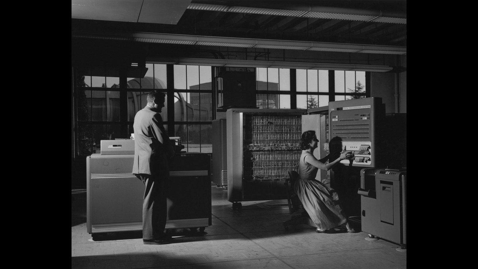
The computing environment deserves a paragraph of its own. UCLA’s own computer in the early 1960s was not powerful enough to run a GCM. Mintz arranged, through his administrative channels, weekend access to the IBM 709 at the UCLA Business School. The 709 had 32 000 words of core memory. A GCM run, at the time, consumed most of that. The model could be compiled in FORTRAN (by 1961 FORTRAN IV was shipping, as I wrote about in the Fortran series), but Arakawa frequently descended to the machine code layer to optimise inner loops. “We cannot afford to do a mistake,” he recalled in 1997. “If there was some drastic error, then an hour is wasted.” When he discovered that he had punched a card wrong, he would pull the card out, scotch-tape over the wrong holes, punch the corrections through the tape by hand, and feed the card back through the reproducer.9 The man who would later invent the mathematical machinery that every digital twin of the planet now runs on spent many of his nights in Los Angeles manually taping IBM punched cards.
Arakawa’s first UCLA stay was brief. His fellowship was a J-1 visa, which under U.S. law required him, at the end of his two years, to return to his home country for two years before he could apply for permanent residency. In 1963 he went home to Japan. Mintz, distraught at the prospect of losing his numerical partner, began writing.
“I really couldn’t make up my mind,” Arakawa told Paul Edwards in the 1997 oral history. “But Mintz wrote me every month!” He remembered a particular moment of decision. His son, then just turned five, was being interviewed for admission to a Tokyo kindergarten. The interviewers showed the boy pictures of animals. He could name each of them – but only in English. The kindergarten declined to admit him. “At that point,” Arakawa said, “I thought, well, my boy, you know, already started his education here in Los Angeles.”9 The family returned to Los Angeles in 1965. Arakawa was given a permanent position on the UCLA faculty. Mintz had his numerical engineer back.
The partnership would continue for twenty-six more years, until Mintz’s death.
Arakawa’s Jacobian
The problem Phillips had described in 1959 – nonlinear computational instability, aliasing of kinetic energy into the smallest resolved scales – was not obvious how to fix. You could not simply add dissipation to damp out the small-scale wiggles, because the real atmosphere has almost no dissipation at those scales (nor does the ocean). Adding artificial smoothing meant lying about the physics. What Arakawa wanted was a finite-difference scheme that was, by mathematical construction, unable to accumulate energy at the grid scale – one whose conservation properties matched those of the continuous equations the model was trying to solve.
The key insight came from two-dimensional fluid dynamics. In the continuous limit, the Jacobian operator that governs advection of vorticity by flow has two exact conservation laws: it conserves total kinetic energy, and it conserves total enstrophy – the spatial integral of the square of the vorticity. Conservation of both is what prevents the unbounded transfer of energy to small scales that Phillips had identified. Most finite-difference approximations to the Jacobian conserve energy. Some conserve enstrophy. Arakawa designed a scheme, in 1966, that conserved both simultaneously.10
The idea looks deceptively simple once you know it. Arakawa’s Jacobian is an average of three different discretisations of the continuous operator, each of which has different conservation properties. The particular linear combination – one third of each – turns out to preserve energy, enstrophy, and the mean vorticity of the flow, all at the same time. Once the scheme preserves those quantities at every time step, the solution cannot drift off to grid-scale infinity. The model stops blowing up.
Arakawa first presented the scheme at a conference in 1962. He published it formally in 1966 in the inaugural issue of the Journal of Computational Physics.11 The paper became one of the most cited articles of the journal’s history, and in 1997, for the journal’s fiftieth-anniversary issue, the editors asked Arakawa to contribute a new commentary and reprinted the original paper alongside it. By that point the Jacobian was appearing in engineering journals that Arakawa said he had never heard of. “It was amazing,” he told Edwards, “the number of citations I got in many kinds of engineering journals that I never saw.”12
The reception at the time was not uniformly enthusiastic. Several senior atmospheric scientists objected that conservation of enstrophy is not a property of the real atmosphere – turbulence does dissipate enstrophy, particularly at high wavenumbers. To build a scheme that rigidly conserves it, they argued, was to enforce a fiction. Arakawa’s response – patient, as it always was – was that the scheme did not claim to be dissipation-free. It claimed to be the right starting point for a model that would then have dissipation added to it by design (eddy viscosity, hyper-diffusion, whatever was physically motivated). What he refused to tolerate was a scheme whose uncontrolled, unphysical dissipation (or worse, uncontrolled accumulation) was a numerical accident rather than a modelling choice. Every model after 1966 would inherit this philosophy: the numerics should be as clean and conservative as possible, and the physics should be added knowingly.
It was Mintz who named the scheme.
Mintz – the senior American collaborator, the one who had recruited Arakawa, the one running the project – could have called the scheme “the Mintz-Arakawa Jacobian” or “the UCLA Jacobian” or any number of other names that would have shared some of the credit. He insisted, instead, that it was Arakawa’s Jacobian. That is what it has been called, in every subsequent textbook, every modeler’s vocabulary, every atmospheric-science PhD thesis that covers numerical methods, for the last sixty years. It is one of the most generous acts of attribution in the history of the discipline.13
The Grids
Arakawa’s second great contribution was on where to put things.
In a numerical model of the atmosphere, you have to decide, at every grid cell, where the variables live. The horizontal wind has two components, u (east-west) and v (north-south). Pressure, temperature, humidity, and other thermodynamic variables are scalars. The vertical velocity is another scalar. Where do you place each of these on the grid? At the centre of the cell? At the corners? At the edges? Does u live at a different place from v?
The choices matter enormously. If u, v, and the scalars all live at the same point – the simplest choice, which Arakawa called the A-grid – then the finite-difference equations for pressure gradient, Coriolis force, and mass continuity are easy to write but resolve short-scale gravity waves badly. Small-amplitude gravity waves in the ocean or the stratosphere, which carry real physical information about wave propagation, get misrepresented as false stationary patterns. The A-grid is numerically simple but physically misleading.
Arakawa understood this by the late 1960s. With his collaborator Vivian Lamb – a UCLA computer scientist who was not, despite the name, the atmospheric modeller – he worked out a systematic catalogue of alternatives. Their 1977 paper in the Methods in Computational Physics series, titled “Computational Design of the Basic Dynamical Processes of the UCLA General Circulation Model,” laid out five grid configurations, labelled A through E, each with different placements of u, v, and the scalars.14

The B-grid, which UCLA used in its own GCM from 1965 onwards, places scalars at the centre of each cell and both wind components together at the cell corners. It handles the Coriolis force naturally and conserves energy well, and Mintz and Arakawa’s model ran on it through the 1970s.
The C-grid, which Arakawa and Lamb found to be the best choice for most applications, places scalars at the cell centre, u at the left and right cell faces, and v at the top and bottom faces – so the two components of the wind are at different locations. The C-grid represents gravity waves correctly, conserves mass well, and handles the geostrophic adjustment process (the way the atmosphere adjusts pressure and wind to be in balance) without producing the spurious wiggles the A-grid generates. In 2026 the C-grid is the default in the Weather Research and Forecasting model (WRF) used by thousands of research groups, in the MIT general circulation ocean model (MITgcm), in the NEMO ocean model used by ECMWF for coupled forecasting, in the Modular Ocean Model (MOM) used by GFDL and most major climate centres, and in about three-quarters of the other numerical models of geophysical fluids that matter. When a graduate student in 2026 writes a new research code for the atmosphere or the ocean, they almost always put their variables on an Arakawa C-grid without thinking hard about it. It is the default.
The D-grid is a rotated version of the C-grid, the E-grid is a further rotation of 45 degrees, and both have their niches (Eta used the E-grid; some finite-element codes have descendants of the D-grid). Which grid to use depends on what you are trying to resolve most carefully – gravity waves, vortices, mass conservation, the Coriolis effect – and on how you want the grid to interact with the model’s spherical geometry. The modern move to cubed-sphere meshes and icosahedral meshes in global models has added a second layer of complication on top of Arakawa’s original choices, but the underlying question – where do u, v, and the scalars live on each mesh cell? – is still, in 2026, the Arakawa question.
The Clouds
Arakawa’s third major contribution was about something that does not happen at the grid scale at all. In the early 1970s, a GCM had grid cells roughly two hundred kilometres across. A cumulus cloud – the convective blob of upward-moving air that produces a thunderstorm – is, typically, ten kilometres across or smaller. A grid cell in a GCM therefore contains, at any given moment, anywhere from zero to several dozen cumulus clouds, none of them resolved. The GCM needs to know what those unresolved clouds are doing – how much heat they transport upward, how much moisture they condense into rain, how much radiation they interact with – without being able to see them individually. Predicting the effect of sub-grid-scale processes on the grid-scale flow is called parameterisation, and the parameterisation of cumulus convection was, through the 1960s and 1970s, one of the hardest unsolved problems in atmospheric modelling.
Arakawa’s approach, developed with his graduate student Wayne Schubert and published in 1974 in the Journal of the Atmospheric Sciences, was called convective quasi-equilibrium. The idea is approximately this. The atmosphere at any given moment is being destabilised by large-scale processes – radiative cooling aloft, surface heating below, moisture transport from the oceans. Convection, when it occurs, stabilises the atmosphere by transporting heat upward. If the destabilisation process is slow compared to the lifetime of a cumulus cloud (about an hour), then convection will adjust, statistically, so that the stabilisation tendency exactly cancels the destabilisation tendency. This means that the ensemble of cumulus clouds in a given grid cell is, on average, in a steady state with respect to the large-scale forcing. If you can work out what forcing the model is applying to a grid cell, you can compute what the cumulus ensemble must be doing to keep the grid cell in statistical equilibrium – without having to simulate the individual clouds at all.15
The Arakawa-Schubert scheme was a major advance. It was based on physical reasoning rather than empirical fitting, and it could predict the altitude distribution of convective heating, the cloud-top height spectrum, and the upward mass flux in a way that purely empirical schemes could not. By the end of the 1970s it was running in the UCLA GCM, in NASA’s GISS model under James Hansen (which was a direct descendant of the UCLA model), and in operational models at several weather centres.
The scheme’s adoption outside UCLA was, in the long run, only partial. The ECMWF operational model under Martin Tiedtke moved, in 1989, to a simpler mass-flux approach that was easier to tune and easier to run. NCAR’s CCM moved, under Guang Zhang and Norman McFarlane, to yet another scheme in 1995. Most modern operational models use some descendant of Tiedtke rather than Arakawa-Schubert. But the WRF model’s “Simplified Arakawa-Schubert” scheme remains in active use, and the physical reasoning behind the original scheme – that convection is in statistical quasi-equilibrium with the large-scale forcing – remains one of the central ideas of atmospheric modelling. When ECMWF and NCAR moved away from the Arakawa-Schubert specifics, they did not move away from the Arakawa-Schubert worldview.16
Schubert, after finishing his PhD at UCLA, joined the faculty at Colorado State University in 1973. He stayed there. The Arakawa-Schubert scheme was the first of what would become a long lineage of UCLA atmospheric-science code at CSU, a lineage that would grow when Arakawa’s student David Randall brought the full UCLA general circulation model there in 1988.
The Lineage
The UCLA GCM itself went through four major versions across the Mintz-Arakawa years: a two-level prototype in 1961-1965 running on an IBM 709 and then on an IBM 360; UCLA I, completed in 1965 and running through the early 1970s on a four-by-five-degree B-grid; UCLA II, with three and nine vertical levels, which was transferred to the NASA Goddard Institute for Space Studies in New York in 1972 and became the starting point for James Hansen’s GISS model; UCLA III, developed in the mid-1970s with twelve levels and a C-grid, which went to the U.S. Navy’s Fleet Numerical Meteorology and Oceanography Center (as the basis for NOGAPS, the operational Navy forecasting model) and to Japan’s Meteorological Research Institute at Tsukuba; and UCLA IV, developed in the late 1970s with an improved planetary boundary-layer and a hybrid vertical coordinate, which David Randall took to Colorado State when he moved there in 1988.17
The UCLA GCM was not the most commercially successful atmospheric model. It did not become an operational forecasting system at a national centre the way Manabe’s model became the backbone of GFDL, or the way Kasahara and Washington’s model evolved into NCAR’s Community Climate Model. What the UCLA GCM did, instead, was travel. Its code, its people, and its numerical schemes went out to the laboratories that became the core of American climate modelling for the next fifty years. James Hansen at GISS in New York. Max Suarez, who joined NASA Goddard’s Global Modeling and Assimilation Office (GMAO) and became its Lead Scientist for Modelling. Lawrence Gates, who took the UCLA model to RAND Corporation and then to Oregon State and ultimately became the founding director of the Program for Climate Model Diagnosis and Intercomparison (PCMDI) at Lawrence Livermore. Wayne Schubert at Colorado State. David Randall at Colorado State, author of the key 2000 reference volume General Circulation Model Development: Past, Present, and Future, coordinating lead author for Working Group I of the IPCC Fourth Assessment Report (which received the 2007 Nobel Peace Prize alongside Al Gore), and – in an act of institutional continuity – the man who brought UCLA IV to CSU and kept it running for another generation of students.
Michael Schlesinger, a UCLA student, collaborated with Mintz on the first three-dimensional stratospheric-ozone transport model in the late 1960s and went on to Oregon State and the University of Illinois. Joao Teixeira, another Arakawa student, went to NASA’s Jet Propulsion Laboratory and is now one of the leading figures in boundary-layer and shallow-convection parameterisation. Steve Krueger at the University of Utah became a pioneer of cloud-resolving modelling. Young-Joon Kim at the U.S. National Weather Service co-developed, with Arakawa, the Kim-Arakawa gravity-wave-drag scheme, which is still used in NOAA operational forecasting.
If there is a single modern American atmospheric scientist who did not in some way drink from the UCLA well, I have trouble naming them. The UCLA GCM did not win the commercial race. It won, decisively, the intellectual one.
There is one branch of the UCLA lineage that is not widely known outside planetary science, and that I want to pause on. In the mid-1960s, while Arakawa was still refining the terrestrial GCM, Mintz began a parallel project with a UCLA graduate student named Conway Leovy. Leovy was interested in Mars. The only reliable information about the Martian atmosphere at the time came from telescopic observation of the polar caps and dust storms. Mariner 4 had flown past Mars in July 1965 and returned a handful of pictures showing a surface that looked, disappointingly, like the Moon. Mariner 9 would not arrive at Mars until 1971 and would not begin to produce the first comprehensive atmospheric observations until after its dust-storm survey. But Mintz and Leovy realised something. The primitive equations that governed the Earth’s atmosphere – the Navier-Stokes equations adapted for a rotating planet, with thermodynamics and moisture physics – are the same equations that govern any planetary atmosphere. If you change the rotation rate, the solar forcing, the atmospheric composition, and the surface topography, you can run the UCLA GCM on Mars.
They did. The Mintz-Leovy Mars GCM, first described in papers in the mid-1960s and formalised through the late 1960s, was the first attempt to apply a full terrestrial general circulation model to another planet. It preceded Mariner 9 by several years. It made predictions that Mariner 9 would then partially confirm: that Mars should have a strong Hadley-like meridional circulation, that polar cap sublimation should drive large seasonal pressure cycles, that dust storms should couple to the atmospheric circulation through radiative heating. Those predictions turned out, broadly, to be right. When NASA’s later Mars Global Surveyor and Mars Reconnaissance Orbiter missions produced detailed atmospheric data in the 2000s, they were compared against successors of the Mintz-Leovy GCM. Planetary meteorology – the discipline that now runs general circulation models of Mars, Venus, Titan, Jupiter, Saturn, and the exoplanets – traces its lineage directly to a UCLA office in 1965. Conway Leovy went on to lead atmospheric sciences at the University of Washington and became the central figure in American Mars meteorology for the next forty years. Mintz, characteristically, never made much of the fact that his UCLA GCM had been the first to leave Earth.
The UCLA GCM also had, from early on, an ambition that was unusual for its era. Mintz was pushing, as the UCLA In Memoriam notes, for coupled ocean-atmosphere modelling “as early as in the late 1960s.” This was ahead of the field. Manabe and Kirk Bryan at GFDL would publish the first coupled ocean-atmosphere GCM paper in 1969. But UCLA was working on similar ideas in parallel, even if its coupled runs did not lead to the same institutional prominence. The question of how the atmosphere and ocean should exchange heat, momentum, and moisture is, in 2026, one of the central questions of climate modelling, and Mintz had pushed it onto the UCLA research agenda half a century ago.
The Charney Report
In the summer of 1979, the U.S. National Research Council asked Jule Charney – who I have written about before in this series, as the man who made the ENIAC forecast work – to chair an ad hoc study group on carbon dioxide and climate. The question the National Research Council wanted answered was simple: if atmospheric CO2 doubles from its pre-industrial value, what will happen to the Earth’s surface temperature?
Charney assembled a panel of eight scientists: himself as chair, D. James Baker of the Joint Oceanographic Institutions, Bert Bolin of Stockholm, Robert Dickinson of NCAR, Richard Goody of Harvard, Cecil Leith of NCAR, Henry Stommel of Woods Hole, Carl Wunsch of MIT – and, as the sole representative of the atmospheric-modelling community, Akio Arakawa. Syukuro Manabe and James Hansen attended as outside experts and briefed the panel on what their respective GCMs were producing. The panel met at Woods Hole from July 23 to 27, 1979.
Yale Mintz was not on the panel. It is not clear from the record whether Charney had invited him and he had declined, or whether he was passed over in favour of his more mathematically oriented younger colleague. Both interpretations are plausible.
The panel’s conclusion, which Charney’s committee delivered in a short report that was shorter than most single chapters of a modern IPCC assessment, was that the equilibrium surface warming for a doubling of CO2 was approximately three degrees Celsius, plus or minus one and a half degrees. The central estimate was a synthesis of the models Manabe had run at GFDL and the models Hansen had run at GISS, the latter being a direct descendant of the UCLA code. Arakawa, in his 1997 oral history, described the panel’s working style: “We kind of tried to start from some skepticism and tried to find something wrong… The panel conclusion was that we were not able to find missing negative feedback, so although we cannot say that the results are right, we didn’t find anything wrong.”18
The three-degree estimate has proven, in the forty-six years since, remarkably robust. The 2021 Intergovernmental Panel on Climate Change Sixth Assessment Report estimates the equilibrium climate sensitivity, after decades of additional modelling, at a likely range of 2.5 to 4 degrees Celsius with a best estimate of 3 degrees. It is the same number. It was produced, the first time, on models whose numerical core had been written by a former Japanese fireman in a quiet UCLA office.
Mintz in Jerusalem
Yale Mintz retired from UCLA in 1977. He was sixty-one. He did not stop working. He moved across the country to NASA’s Goddard Space Flight Center in Greenbelt, Maryland, where Milton Halem (one of the UCLA GCM’s early collaborators) hosted him as a consulting scientist. His Goddard years were productive. Freed from the administrative demands of a UCLA chair, he turned his attention to something that had been neglected in the first generation of GCMs: the land surface.
The early UCLA, GFDL, and NCAR models treated the land surface as a simple thermal bucket. Soil moisture was either prescribed or ignored. Vegetation was a roughness length. Evapotranspiration, the process by which water evaporates from soil and transpires from leaves, was handled by a few tuning parameters. Mintz, in his Goddard years, showed that this treatment was badly wrong. With Jagadish Shukla – then at the University of Maryland, later at George Mason, and one of the leading climate dynamicists of his generation – Mintz published a 1982 paper in Science titled “Influence of Land-Surface Evapotranspiration on the Earth’s Climate” that demonstrated, using a pair of UCLA GCM experiments with and without realistic soil moisture, that the treatment of the land surface matters enormously for simulated precipitation patterns worldwide.19 The paper was an early, influential statement of what would become a major research programme at GFDL, NCAR, ECMWF, and the Hadley Centre through the 1980s and 1990s: the land surface is a fully-featured component of the climate system, not an afterthought.
From the mid-1970s onwards Mintz took sabbatical quarters in Israel, at the Hebrew University and the Weizmann Institute. His connections there deepened. In his last years he moved to Jerusalem.
He died there on April 27, 1991, at the age of seventy-five, after what his UCLA colleagues described as “several months of a brave fight against cancer.”20 The UCLA In Memoriam, written by Arakawa, S. V. Venkateswaran, and Mort Wurtele, ended with a sentence that captures the man: “Yale Mintz was religious by temperament, liberal and international in outlook, and an academic by choice.” He had received the Carl-Gustaf Rossby Research Medal from the American Meteorological Society the year before his death, in 1990 – the society’s highest honour, given for “preeminent leadership in the global modelling of climate, and for inspiring tutelage of several generations of scientists.” He had been, in the opinion of the UCLA In Memoriam authors, one of the most generous scientists of his generation: a man who never wrote a line of code but who insisted, again and again, that the schemes his colleague had invented be named after his colleague alone.
Arakawa’s Last Thirty Years
After Mintz’s death, Arakawa continued at UCLA for another three decades. He was by then sixty-four. He kept teaching. He kept publishing. His 1997 paper for the Journal of Computational Physics fiftieth-anniversary issue – a new commentary on the original 1966 Jacobian paper – was one of the last systematic retrospective pieces he wrote. His 2000 contribution to David Randall’s edited volume General Circulation Model Development was the summary of modern GCM design from the man who had invented most of it.
His students fanned out across the discipline. Wayne Schubert at Colorado State was joined, in 1988, by David Randall, who brought UCLA IV with him. At NASA Goddard, Max Suarez built the modelling capacity that would become GMAO. At JPL, Joao Teixeira worked on boundary-layer parameterisation. At the University of Utah, Steve Krueger pioneered cloud-resolving models. A group photograph from January 2014 at UCLA shows Arakawa, eighty-six, in the centre of a crowd of former students, collaborators, and their students in turn – four academic generations of climate modellers standing around the man who had, in 1961, been brought across the Pacific to fix a mathematical problem that threatened to make the whole enterprise unworkable.
There is one more comparison worth drawing. The post on Manabe and the GFDL Nobel I wrote earlier in this series tells a story about a different Japanese-born American meteorologist who was, in many ways, Arakawa’s opposite number. Syukuro Manabe and Akio Arakawa were born two years apart (Manabe 1931, Arakawa 1927), left Japan for the United States within a few years of each other, and spent the following six decades building the two most influential atmospheric modelling programmes in the world: Manabe at GFDL in Princeton, Arakawa at UCLA in Los Angeles. They knew each other. They respected each other. They worked in the same small community and were invited to the same conferences. Their approaches to the work were very different. Manabe was, above all, a physicist: his emphasis was on getting the radiative transfer right, the water vapour feedback right, the vertical profile right. Manabe built models that produced climate predictions, and the predictions were right. Arakawa was a mathematician: his emphasis was on getting the numerics right, the grid right, the conservation laws right. Arakawa built models that produced climate predictions, and the predictions were stable. Both things matter. The Nobel Prize went, in 2021, to Manabe. The methodology it was built on, including the schemes Manabe’s own code uses for the advection of vorticity, came from Arakawa. It is a rare configuration in science that two co-Nobels would genuinely be deserved. Had a Nobel Prize existed for computational meteorology in some parallel universe, Arakawa would have shared it.
Arakawa remained in Los Angeles. His wife and his son (whose 1963 failure of the Tokyo kindergarten interview had decided the family’s geography) and his grandson and granddaughter were there. He travelled occasionally to Japan to see family and to Europe to lecture. In his later years he was a regular guest at seminars and at memorial meetings; he could, at age ninety, still hold a lecture room’s attention for two hours on the history of numerical methods.
He died on March 21, 2021, in Los Angeles, at the age of ninety-three. The UCLA Department of Atmospheric and Oceanic Sciences obituary, which appeared four days later, said he had died at home while sleeping.21 In October 2022 a two-day Arakawa Symposium at UCLA, organised by Roger Wakimoto, Rong Fu, and David Randall, brought several dozen of his students and intellectual heirs together to trace the scientific lineage one more time. The symposium programme’s roster of speakers reads like a who’s-who of modern atmospheric modelling. Almost every speaker on it had, at some point in their career, run code whose mathematical infrastructure was Arakawa’s.
What They Built
It is a strange thing to be a mathematician whose work lives inside the programs of other people. Arakawa wrote relatively few papers – his obsessive standards kept his publication list short. The papers he did write are all, at this point, half a century old or older. The 1966 Jacobian paper is sixty years old. The 1974 convection paper is fifty-two. The 1977 grids paper is forty-nine. And yet, in 2026, every atmospheric model in operational use and almost every ocean model employs mathematical schemes that are either direct implementations of what those papers describe or lineal descendants of them.
Arakawa’s Jacobian, in various forms, is in the dynamical cores of the ECMWF IFS, NOAA’s FV3, NCAR’s CAM, and a dozen smaller models. Arakawa C-grids are in WRF, MITgcm, NEMO, MOM, ROMS (the Regional Ocean Modeling System), and ICON (the German DWD model). The convective quasi-equilibrium idea that Arakawa and Schubert formalised in 1974 has been modified and extended but not really superseded; every parameterisation since has had to say something about what balance or lack thereof exists between convective and large-scale forcings. A climate simulation of the twenty-first century that shows what happens to the tropics under four degrees of warming is being run on mathematical scaffolding that Arakawa designed in his UCLA office between his first visit in 1961 and his 1977 retirement as chair.
There are a handful of contributions in the history of computational science that have this kind of quiet, pervasive presence. Dijkstra’s algorithms. Kalman’s filter. Backus’s BNF. Nozaki’s singular-value decomposition. Wilkinson’s numerical linear algebra. These are the mathematical objects that everyone uses and few can name. Arakawa’s work belongs in that small group.
It is useful, if you are interested in the topic of this blog – the history of weather and climate prediction – to remember the following. Numerical weather prediction is, from one angle, a story of machines: ENIAC, IBM 704, IBM 7090, CDC 6600, Cray-1, and their successors. From another angle, it is a story of atmospheric physics: the primitive equations, the jet stream, the Madden-Julian oscillation, the stratospheric ozone layer, the coupling between the atmosphere and the ocean. From a third angle, and this is Arakawa’s angle, it is a story of numerical methods – of the unglamorous, painstaking work of building finite-difference schemes that conserve the right things, that place the variables in the right places, that handle sub-grid-scale processes without blowing up the large-scale solution.
If the machines had been available without the physics, they would have produced nothing. If the physics had been worked out without the machines, they would have produced only papers. If the machines and the physics had come together without the numerical methods, the simulations would have run for thirty simulated days and then exploded, as Phillips’s did in 1956. The reason the ECMWF IFS can today produce a ten-day forecast whose 500-hectopascal geopotential height fields verify against observations at a correlation of 0.90 is that all three legs – machine, physics, and numerics – got built.
Arakawa built the third leg. Mintz made it possible for him to do so. The first two legs we have covered in other posts of this series and will cover again. For today, it is enough to say that the most consequential partnership in the history of atmospheric numerical methods was between a Brooklyn-born Dartmouth humanist who never learned to program and a Tokyo-born former wartime fireman who, after his first thermometer was lost on the Pacific floor, spent the next seventy years making sure nothing else he built would break under pressure.
Footnotes
References
Primary sources:
- Arakawa, A. (1966). “Computational Design for Long-Term Numerical Integration of the Equations of Fluid Motion: Two-Dimensional Incompressible Flow. Part I.” Journal of Computational Physics 1(1), 119-143.
- Arakawa, A., and Lamb, V. R. (1977). “Computational Design of the Basic Dynamical Processes of the UCLA General Circulation Model.” Methods in Computational Physics 17, 173-265.
- Arakawa, A., and Schubert, W. H. (1974). “Interaction of a Cumulus Cloud Ensemble with the Large-Scale Environment, Part I.” Journal of the Atmospheric Sciences 31(3), 674-701.
- Mintz, Y. (1951). “The geostrophic poleward flux of angular momentum in the month of January 1949.” Tellus 3, 195-200.
- Mintz, Y. (1954). “The observed zonal circulation of the atmosphere.” BAMS 35(5), 208-214.
- Phillips, N. A. (1956). “The general circulation of the atmosphere: a numerical experiment.” QJRMS 82, 123-164.
- Phillips, N. A. (1959). “An example of non-linear computational instability.” In B. Bolin (ed.), The Atmosphere and the Sea in Motion (Rossby Memorial Volume), Rockefeller Institute Press, 501-504.
- Shukla, J., and Mintz, Y. (1982). “Influence of Land-Surface Evapotranspiration on the Earth’s Climate.” Science 215, 1498-1501.
- Charney, J. G. et al. (1979). Carbon Dioxide and Climate: A Scientific Assessment. National Academy of Sciences.
- Tiedtke, M. (1989). “A comprehensive mass flux scheme for cumulus parameterization in large-scale models.” Monthly Weather Review 117, 1779-1800.
Oral histories and memoirs:
- Arakawa, A. Oral history interview with Paul N. Edwards, 17-18 July 1997. AIP Niels Bohr Library Session I; Session II.
- Johnson, D. R., and Arakawa, A. (1996). “On the Scientific Contributions and Insight of Professor Yale Mintz.” Journal of Climate 9(12), 3211-3224.
- University of California. In Memoriam, 1993: Yale Mintz, Atmospheric Sciences, Los Angeles, 1916-1991. Authors: Akio Arakawa, S. V. Venkateswaran, Morton G. Wurtele.
Biographical and secondary:
- Akio Arakawa – Wikipedia.
- Arakawa grids – Wikipedia.
- UCLA Department of Atmospheric and Oceanic Sciences: Arakawa memorial page, 2021; department history; Arakawa Symposium, October 2022.
- Weart, S. “Arakawa’s Computation Device.” The Discovery of Global Warming, American Institute of Physics. Link.
- Edwards, P. N. (2010). A Vast Machine: Computer Models, Climate Data, and the Politics of Global Warming. MIT Press. UCLA chapter online at pne.people.si.umich.edu.
- Randall, D. A. (ed.) (2000). General Circulation Model Development: Past, Present, and Future. Academic Press.
Charney Report:
Cross-references in this series:
- The First Climate Model Had 5KB of RAM – Phillips’s 1956 experiment.
- The Man Who Tamed the Equations – Charney and the 1950 ENIAC forecast.
- The Line That Models Cannot Draw – the Bergen School and Jacob Bjerknes.
- The Forecast That Reached the Nobel – Manabe and the GFDL models.
- God Is Real (Unless Declared Integer) – beginning of the Fortran miniseries, the language that runs all of this.
-
Arakawa, A. Oral history interview with Paul N. Edwards, 17 July 1997 (Session I). AIP Niels Bohr Library. ↩
-
Arakawa, A. Oral history, same reference as footnote 1. ↩
-
Phillips, N. A. (1959). “An example of non-linear computational instability.” In The Atmosphere and the Sea in Motion: Scientific Contributions to the Rossby Memorial Volume, B. Bolin (ed.), Rockefeller Institute Press, 501-504. Also discussed in Phillips’s 1956 QJRMS paper on the two-level general circulation experiment, which I have covered in my earlier post on The First Climate Model. ↩
-
University of California. In Memoriam, 1993: Yale Mintz, Atmospheric Sciences, Los Angeles, 1916-1991. Authors: Akio Arakawa, S. V. Venkateswaran, Morton G. Wurtele. Web archive version. ↩
-
Johnson, D. R., and Arakawa, A. (1996). “On the Scientific Contributions and Insight of Professor Yale Mintz.” Journal of Climate 9(12), 3211-3224. AMS Journals link. Mintz, Y. (1951). “The geostrophic poleward flux of angular momentum in the month of January 1949.” Tellus 3, 195-200. Mintz, Y. (1954). “The observed zonal circulation of the atmosphere.” BAMS 35(5), 208-214. ↩
-
UCLA In Memoriam 1993, same reference as footnote 4. ↩
-
Arakawa oral history, 1997, same reference as footnote 1. ↩
-
Weart, S. “Arakawa’s Computation Device.” The Discovery of Global Warming (AIP history archive). Link. ↩
-
Arakawa oral history, 1997, same reference as footnote 1. ↩ ↩2
-
The mathematical details are in Arakawa’s 1966 paper; a readable secondary account is in Randall, D. A. (2000). General Circulation Model Development: Past, Present, and Future. Academic Press. Chapter 1 (Arakawa’s own contribution) is a useful primer. ↩
-
Arakawa, A. (1966). “Computational Design for Long-Term Numerical Integration of the Equations of Fluid Motion: Two-Dimensional Incompressible Flow. Part I.” Journal of Computational Physics 1(1), 119-143. ↩
-
Arakawa oral history, 1997, same reference as footnote 1. ↩
-
UCLA In Memoriam 1993, same reference as footnote 4. The naming of the Jacobian is explicit in Arakawa’s 1996 tribute to Mintz (co-authored with Johnson), see footnote 5. ↩
-
Arakawa, A., and Lamb, V. R. (1977). “Computational Design of the Basic Dynamical Processes of the UCLA General Circulation Model.” Methods in Computational Physics 17, 173-265. Academic Press. ↩
-
Arakawa, A., and Schubert, W. H. (1974). “Interaction of a Cumulus Cloud Ensemble with the Large-Scale Environment, Part I.” Journal of the Atmospheric Sciences 31(3), 674-701. ↩
-
Tiedtke, M. (1989). “A comprehensive mass flux scheme for cumulus parameterization in large-scale models.” Monthly Weather Review 117, 1779-1800. Zhang, G. J., and McFarlane, N. A. (1995). “Sensitivity of climate simulations to the parameterization of cumulus convection in the Canadian Climate Centre general circulation model.” Atmosphere-Ocean 33, 407-446. ↩
-
Paul N. Edwards. A Vast Machine: Computer Models, Climate Data, and the Politics of Global Warming. MIT Press (2010). Chapter on the UCLA GCM available at pne.people.si.umich.edu/vastmachine/i.UCLA.html. ↩
-
Arakawa oral history, 1997, same reference as footnote 1. Charney, J. G. et al. (1979). Carbon Dioxide and Climate: A Scientific Assessment. National Academy of Sciences. ↩
-
Shukla, J., and Mintz, Y. (1982). “Influence of Land-Surface Evapotranspiration on the Earth’s Climate.” Science 215, 1498-1501. ↩
-
UCLA In Memoriam 1993, same reference as footnote 4. ↩
-
UCLA Department of Atmospheric and Oceanic Sciences. “Dr. Akio Arakawa, Distinguished Research Professor Emeritus” (25 March 2021). Link. ↩