The ocean is much harder to simulate than the atmosphere. This is not because the equations are different; they are not. Both fluids are governed by the same Navier-Stokes system, the same thermodynamics, the same rotating-reference-frame physics. What makes the ocean harder is time.
The atmosphere and the ocean both support two broad classes of motion. The fast motions are acoustic and gravity waves that propagate at hundreds of metres per second, limited by the speed at which pressure disturbances travel. A sound wave in the atmosphere takes a few seconds to cross a kilometre; a surface gravity wave in the ocean, in deep water, does something similar. The slow motions are the large-scale circulation patterns that carry heat and water around the planet: the jet stream, the Gulf Stream, the meridional overturning. Those move at centimetres to metres per second. They evolve over days in the atmosphere and over years, centuries, or millennia in the ocean.
On a computer, this mixture of fast and slow is an expensive problem. The Courant-Friedrichs-Lewy condition says that a numerical time step must be shorter than the time a fast wave takes to cross a grid cell. If the fast waves are minutes apart, the time step has to be a few minutes. If the system you care about equilibrates in a thousand years, the simulation has to take a hundred million time steps. On a 1969 UNIVAC 1108, with a half-megabyte of core memory and a floating-point speed measured in tens of thousands of operations per second, a hundred million time steps was not a thing you could do. It was not even close.
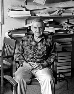
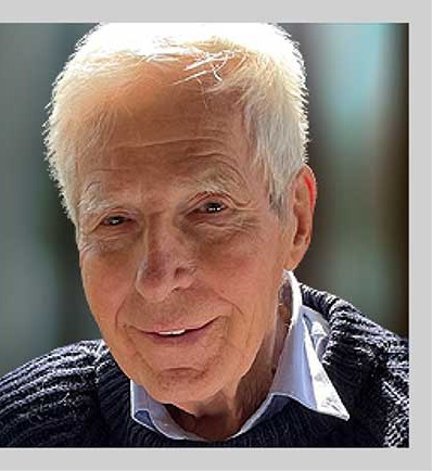
This post is about the man who figured out how to do it anyway. His name is Kirk Bryan. He is ninety-six years old, still listed on the Princeton faculty roster, and in 2023 he accepted the Alexander Agassiz Medal from the National Academy of Sciences in person at the age of ninety-three. In 1969 he published a twenty-nine-page paper in the inaugural years of the Journal of Computational Physics that invented numerical ocean modelling. He also, that same year, co-authored with Syukuro Manabe a four-page paper in the Journal of the Atmospheric Sciences that presented the first coupled ocean-atmosphere general circulation model in the history of the field. Manabe would win the Nobel Prize in Physics in 2021 for the lineage of models that paper began. Bryan did not. The mathematical machinery Manabe’s Nobel depends on was Bryan’s.
What follows is the story of how Bryan built the ocean on a half-megabyte computer, what numerical trick let him do it, who helped him, and what happened to the code when he let it out into the world.
Woods Hole, 1951
Kirk Bryan Jr. was born on July 21, 1929, into a family of field scientists. His grandfather Richard Bryan had been an astronomer on the disastrous 1871-73 Polaris expedition to the Arctic, during which his ship was lost and the crew rescued from an ice floe. His father Kirk Bryan Sr. was a Harvard geology professor who specialised in the erosion and hydrology of the American Southwest, and who died suddenly of a heart attack on a field trip in Colorado in August 1950 – three months before his son started his senior year at Yale.1
Bryan Jr. graduated from Yale in 1951 with a bachelor’s degree and no particular idea of what to do with it. What he did, for reasons that his later oral history interviews do not entirely explain, was drive to Woods Hole, Massachusetts, on the Cape Cod coast, and talk his way into a junior research position at the Woods Hole Oceanographic Institution. He spent approximately two years there between 1951 and 1953. His principal scientific influence during those years was a man named Henry Stommel.2
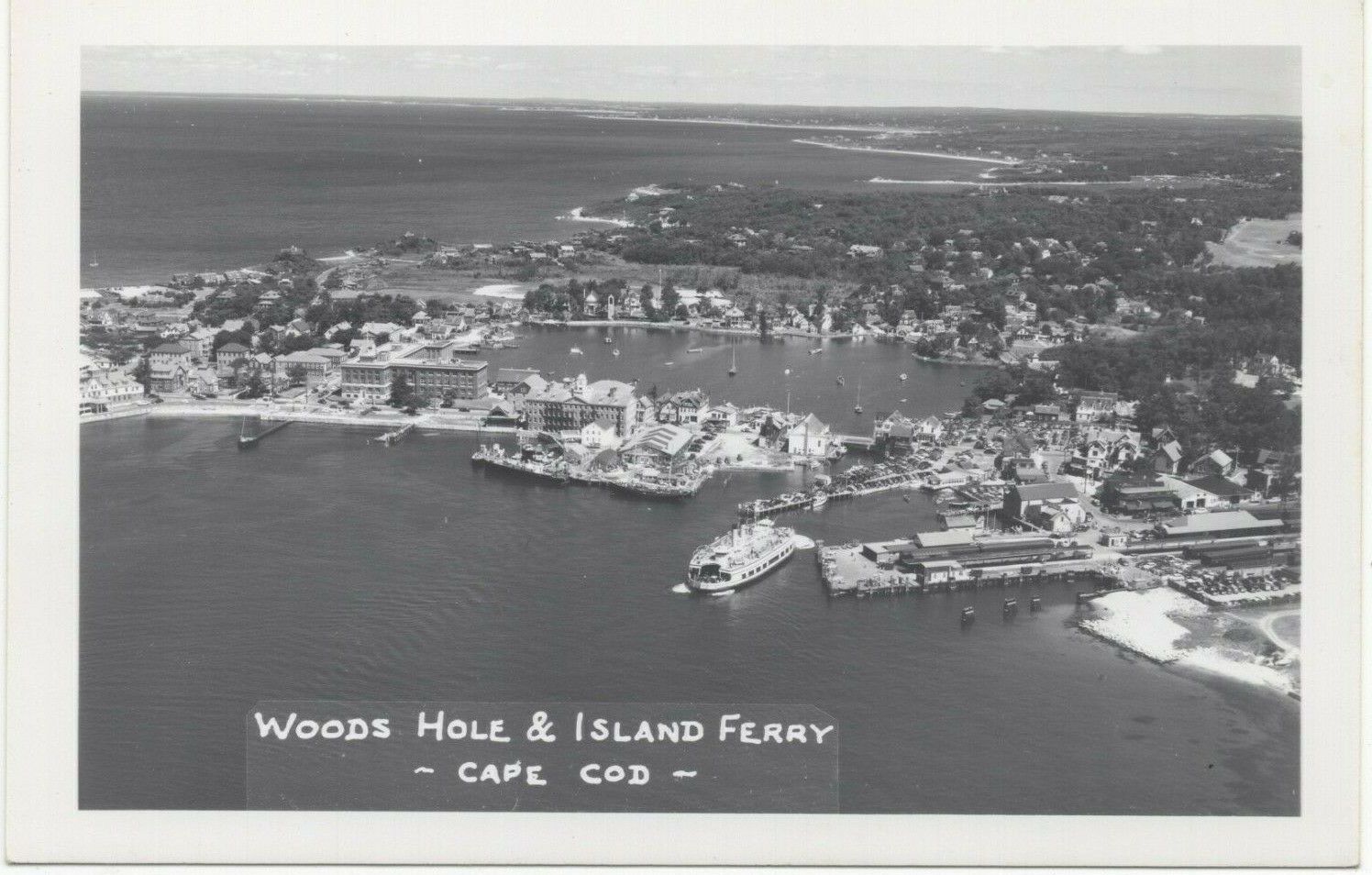
Stommel, at that point thirty-one years old, was the most mathematically original physical oceanographer of his generation. He had published, in 1948, a short paper in the Transactions of the American Geophysical Union titled “The Westward Intensification of Wind-Driven Ocean Currents.” It is one of the great papers in twentieth-century geophysics.3 In three pages and one equation, Stommel explained why the Gulf Stream hugs the east coast of North America and the Kuroshio Current hugs the east coast of Japan, rather than being distributed evenly around the rim of the basin: the Coriolis parameter varies with latitude, and this asymmetry – the beta effect – concentrates the return flow of wind-driven ocean circulation into narrow western boundary currents. Before Stommel, the Gulf Stream was a mystery. After Stommel, it was a theorem.
Stommel was famously sceptical of big numerical codes for most of his career. He preferred elegant pencil-and-paper models, simple enough that one person could hold the whole argument in their head. The ocean-modelling revolution Bryan would launch in the 1960s was, in one sense, exactly the kind of computational brute force Stommel mistrusted. But he had given Bryan something that would shape every line of Fortran Bryan would write for the next sixty years: the conviction that the ocean’s circulation was a well-posed mathematical problem, that the Gulf Stream could be understood rather than merely observed, and that with the right equations and the right boundary conditions you could compute the ocean. Bryan carried that conviction to MIT.
MIT and Lorenz, 1953-1957
Bryan’s PhD work at MIT between 1953 and 1957 was not in oceanography. It was in dynamical meteorology, under Edward N. Lorenz.4 The thesis was titled A numerical investigation of certain features of the general circulation. Lorenz – whose later 1963 paper on chaos I wrote about in the Lorenz post – was in 1953 not yet the founder of chaos theory, but he was already one of the most rigorous mathematical minds in American meteorology. He had been Joseph Smagorinsky’s own teacher at MIT during Smagorinsky’s WWII Army Air Corps training a decade earlier. By Bryan’s time, Lorenz was training a new generation on the same foundation: careful numerical experimentation on the atmospheric primitive equations, under the assumption that computers would soon be powerful enough to run them.
Bryan finished in 1957. He had, by then, the unusual combination that Joseph Smagorinsky was looking for. He had a Woods Hole oceanographer’s training in dynamical ocean theory, courtesy of Stommel. He had an MIT meteorology PhD in numerical methods, courtesy of Lorenz. He had grown up in a Harvard geology family, with a geologist’s feel for planetary time scales. He was twenty-eight years old. Smagorinsky called.
GFDL, 1961
The Geophysical Fluid Dynamics Laboratory in 1961 was not called GFDL yet. It was the General Circulation Research Laboratory of the United States Weather Bureau, based in Washington, DC, with about a dozen scientists, a hand-wired connection to a borrowed IBM 7030 Stretch, and a plan. The plan had been laid down in 1955 by Joseph Smagorinsky at John von Neumann’s suggestion: a comprehensive numerical model of the Earth’s climate, coupling the atmosphere and the ocean into one integrated simulation. Smagorinsky was forty years old, had co-authored the 1950 ENIAC weather forecast with Charney, and had been running the lab since 1955. He had hired Syukuro Manabe in 1958 to do the atmosphere half. He had nobody for the ocean half.
The hiring problem Smagorinsky faced in 1961 was harder than it sounds. The atmospheric-modelling community in 1961 was small but coherent – a handful of scientists at GFDL, UCLA (where Mintz and Arakawa were starting the UCLA GCM I wrote about yesterday), and NCAR – all of them converging on the same set of numerical techniques for the same primitive equations. The ocean-modelling community, as of 1961, consisted of approximately zero people. There were no ocean general circulation models anywhere in the world. There were dynamical theories – Stommel’s 1948 paper, Walter Munk’s 1950 theory of the Sverdrup transport, Arnold Arons’s work on abyssal circulation – but no numerical codes. The closest anyone had come was Munk’s 1950 analytical solution for wind-driven circulation, which was so idealised that it could be evaluated on a slide rule.
Smagorinsky needed somebody who could take Stommel’s ocean and put it on a computer. The somebody had to know oceanography (from Woods Hole, for preference), know numerical methods (from MIT or one of the three or four other places that taught them), and be young enough to accept what would in 1961 look like a career-risking bet on a new subfield that did not yet exist. Kirk Bryan fit the profile so exactly that it is almost as if Smagorinsky had designed the requirements around him.5
Smagorinsky hired him in 1961. Bryan would lead the GFDL Ocean Division for the next thirty-four years, from 1961 until his retirement in 1995, through the transition from the Weather Bureau to ESSA to NOAA, through the lab’s 1968 move from Washington to Princeton, through the four generations of mainframe computers that would arrive at the new Princeton building, and through every coupled climate model the laboratory would produce from his first day there to the publication of the IPCC First Assessment Report in 1990 for which he was a lead author.6
The First Model, 1963
Bryan’s first ocean-modelling paper appeared in 1963 in the Journal of the Atmospheric Sciences – the journal, not the field, because no Journal of Physical Oceanography yet existed. It was titled “A Numerical Investigation of a Nonlinear Model of a Wind-Driven Ocean.”7 It is a paper that is routinely skipped in summaries of Bryan’s career, in favour of the better-known 1967 Bryan-Cox paper. I want to linger on it, because it is the paper in which Bryan invented the basic numerical machinery that every subsequent ocean model has used.
The 1963 model was intentionally minimal. It had no thermodynamics – no temperature, no salinity, no density variations. The ocean was a single homogeneous fluid. It had no realistic geography – a rectangular basin bounded by straight walls. Its forcing was a simple wind stress at the surface, chosen to mimic the mid-latitude westerlies. What mattered was the machinery Bryan built to simulate it: a set of finite-difference approximations to the primitive equations on a spherical grid, explicit time-stepping with the Euler method, and careful attention to the nonlinear instabilities that had plagued Phillips’s 1956 atmospheric experiment (which I wrote about in the Phillips post). The 1963 model used a variant of the Arakawa B-grid: scalars at cell centres, velocities at cell corners. It used Smagorinsky-style viscosity to control numerical instabilities. It integrated for hundreds of simulated days on an IBM 7030 Stretch.
In the limit where the flow reached a steady state, the 1963 model’s solution reproduced, numerically, the analytical solution Walter Munk and colleagues had derived in 1950 for wind-driven ocean circulation. The Munk solution has the Gulf Stream on the western boundary (by Stommel’s beta effect) and the Sverdrup return flow across the interior. Bryan’s numerical Gulf Stream was not sharper or deeper than Munk’s analytical one, but it was more: Bryan’s was time-dependent, nonlinear, and able to handle flows that analytical methods could not. It was the first working proof that the ocean general circulation could be computed rather than just approximated.
The 1963 paper was a proof of concept. The 1967 paper was the real beginning.
Adding the Density Field: Bryan and Cox, 1967
In 1967 Bryan and a new colleague named Michael Cox published a paper in Tellus titled “A numerical investigation of the oceanic general circulation.”8 The Cox in the co-author line was a young man who had arrived at GFDL not as a scientist but as a computer operator – part of the team that ran the lab’s batch-mainframe jobs, punched cards, mounted tapes. Cox had turned out to have unusual aptitude for the kind of numerical programming Bryan’s ocean model required, and Bryan had pulled him into the research side. He would remain Bryan’s closest collaborator for the next twenty-two years, until his death.9
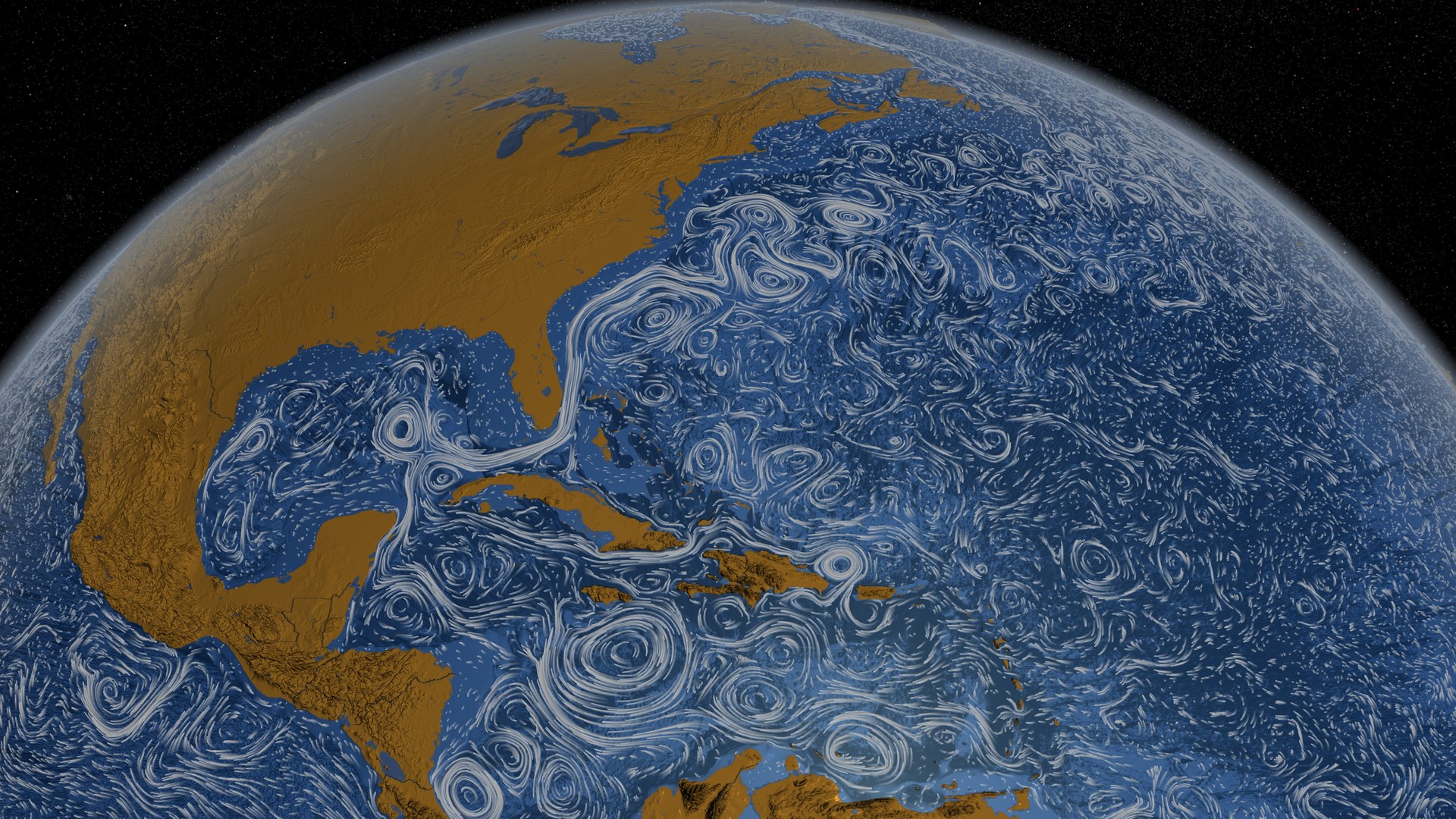
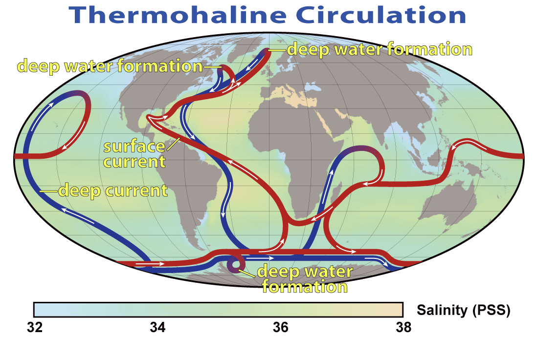
The 1967 Bryan-Cox paper added to the 1963 model what had been missing: buoyancy forcing. The ocean, in reality, is stratified by temperature and salinity. The warm surface waters of the tropics are less dense than the cold deep waters of the polar basins. The density difference drives the global thermohaline circulation – the slow (thousand-year) overturning by which cold dense water sinks in the North Atlantic and the Southern Ocean and flows along the deep abyss, eventually returning to the surface in the upwelling regions of the tropics. Without density, you have a wind-driven ocean but no climate. With density, you have the circulation that transports heat from the equator to the poles, and the circulation that stores most of the excess heat added to the Earth by rising greenhouse gases.
Adding temperature and salinity was not just a matter of adding two more prognostic variables. It required the full primitive-equation ocean system: conservation of mass, momentum, heat, and salt; an equation of state linking temperature, salinity, and pressure to density; parameterisations for vertical mixing of heat and momentum; and boundary conditions at the surface (heat flux, evaporation minus precipitation, wind stress) and the ocean floor (no flow through bathymetry, possible heat flux). The 1967 paper brought all of this together in a three-dimensional, idealised-geometry model running on a spherical grid. The computer was a CDC 6600, which Control Data had begun delivering in 1964, making it the fastest machine in the world.10 GFDL had one. It ran at about three million floating-point operations per second and had 131 thousand sixty-bit words of memory – about a megabyte, by modern reckoning.
The 1967 model could not yet run with real continents. But it had everything else. It produced warm surface waters in the tropics, cold deep water in the polar basins, a wind-driven gyre circulation in mid-latitudes, and a slow thermohaline overturning that carried heat poleward. It was, in miniature, a working ocean.
The Problem of Time
Here I have to explain something that makes ocean modelling specifically, qualitatively different from atmospheric modelling, because it is the problem Bryan solved in 1969 and it is the reason every modern ocean model still contains the ghost of his solution.
A numerical model of a fluid advances in discrete time steps. At each step, the program computes the state of the fluid at the next time from its state at the current time. The Courant-Friedrichs-Lewy condition says that the time step must be shorter than the time it takes the fastest wave in the system to cross one grid cell. If the grid cells are 100 km across, and the fastest wave in the ocean is a surface gravity wave propagating at about 200 metres per second, then the time step has to be less than 500 seconds – call it five minutes. If you run for one simulated day, that is roughly 300 steps. One simulated year is about 100 000 steps. One simulated century is ten million steps.
The ocean’s slow circulation – the thermohaline overturning – takes about a thousand years to spin up from an arbitrary initial condition to a realistic steady state. To run an ocean model to equilibrium you therefore need approximately a hundred million time steps. On a CDC 6600 delivering three million floating-point operations per second, with a three-dimensional grid that requires at least a million operations per step, this works out to about a thousand years of CPU time per simulated millennium. Nobody was going to do that.
This is the problem Bryan faced in the late 1960s. The equations of the ocean were clear. The numerical methods of 1967 worked. But the computer was about a thousand times too slow to integrate a realistic world ocean for long enough to see anything interesting happen. Something had to give.
What gave was the surface gravity wave.
The Rigid Lid
The insight Bryan had – the central algorithmic insight of his entire career, and one of the most consequential design decisions in the history of geophysical fluid dynamics – was that the fast surface gravity wave does not matter for the slow, large-scale circulation of the ocean. It is real, it exists, and it has a role in tsunamis and in the dynamics of the open boundaries of coastal models. But for the question of how the deep ocean overturns, how much heat the Gulf Stream carries poleward, how the circulation redistributes salt – the question of climate – the fast barotropic mode is a messenger carrying information the slow modes already have. If you could delete it from the simulation without losing anything important, you could increase the time step from five minutes to a day, and the 1969 model’s thousand-year spin-up would become computationally possible.
Bryan’s trick for deleting the fast mode was to pretend that the ocean has a rigid top. Normally, the surface of the ocean is free to move: the height of the water responds to the wind and to internal dynamics, and that free surface is what supports gravity waves. Bryan’s 1969 paper took the boundary condition at the top of the ocean and replaced it with w(z=0) = 0: the vertical velocity at the sea surface is exactly zero. This is not physically true. But if you impose it, the fast gravity waves disappear from the equations. What remains are the slow modes, which can be integrated with a daily time step without numerical instability.11
There is no free lunch. Deleting the fast mode introduces a new problem: the horizontal depth-averaged (“barotropic”) flow has to conserve mass somehow. In the real ocean, mass is conserved through changes in the surface height. With a rigid lid, you cannot store mass at the surface; mass conservation becomes a constraint on the horizontal flow. Bryan solved this by introducing a streamfunction for the barotropic flow – a two-dimensional scalar field whose derivatives give the depth-averaged horizontal currents – and solving an elliptic partial differential equation for the streamfunction at every time step. The elliptic solve is expensive but not as expensive as taking a million time steps per day. The net win, when Bryan ran the numbers, was roughly two orders of magnitude. A simulation that would have required a thousand years of CPU time could now be done in tens of years. Coupled ocean-atmosphere runs that would have been impossible became just barely possible.
The rigid-lid approximation ruled ocean modelling from 1969 until the early 1990s. It was replaced by free-surface methods, developed by Peter Killworth and collaborators in the UK in 1991 and by John Dukowicz and Rick Smith at Los Alamos in 1994,12 which handle the free-surface problem implicitly rather than removing it. Modern ocean models (MOM6, NEMO, POP) use free-surface methods. But every free-surface method in use today was designed to reproduce, in the slow-mode limit, the solutions that rigid-lid models had been producing for twenty-five years. The rigid lid is gone. The equations the free-surface methods were built to reproduce are the ones Bryan wrote in 1969.
The 1969 Paper
The paper that made all of this public is “A Numerical Method for the Study of the Circulation of the World Ocean,” Journal of Computational Physics 4(3), 347-376, published in the journal’s inaugural run.13 It is twenty-nine pages long. It presents, for the first time anywhere, the finite-difference approximation of the primitive equations of the ocean on a spherical grid with realistic continental outlines and realistic bathymetry. It introduces the rigid-lid approximation and the streamfunction method. It gives sample solutions for a world ocean forced by realistic wind stresses and surface temperature. It is the founding document of numerical ocean modelling.
It is also, in retrospect, remarkable for how little it flags what it is doing. Bryan presents the rigid-lid approximation in a single paragraph on page 354, as if it were an obvious step in the discretisation. There is no discussion of free-surface alternatives. There is no comparative computing-cost analysis. There is just the equation, the method, and the results. The reader who does not know the problem Bryan is solving will not understand what he has done. Bryan’s entire career, in print, has this quality: papers so spare that the magnitude of what they invent is invisible unless you know what they invented.
The 1969 JCP paper was reprinted in 1997 for the Journal of Computational Physics fiftieth-anniversary issue, with a new commentary by Bryan. That reprint is, as far as I know, the only primary-source discussion by Bryan of what he had done in 1969 and why.14
Four Pages, Half a Megabyte
The same year the JCP paper appeared, Bryan and Manabe published another paper – in the Journal of the Atmospheric Sciences, April 1969, four pages long – titled “Climate Calculations with a Combined Ocean-Atmosphere Model.”15
Two paragraphs in, the paper explains what it is. “The experiments described in this note are made with a numerical model of the atmosphere and the world oceans coupled together.” There was no previous model to compare it to. It was the first of its kind. The atmospheric component was Manabe’s nine-level hemispheric GCM, the one that had produced the 1967 radiative-convective results that would lead, five decades later, to the 2021 Nobel Prize in Physics. The ocean component was Bryan’s five-level model, running with a rigid lid and realistic North Pacific and North Atlantic geometry. The two components exchanged heat, moisture, and wind stress at the surface at every coupled time step.
The computer was a UNIVAC 1108 at Princeton. The UNIVAC 1108, introduced in 1964 and still in production in 1969, was a mid-range scientific mainframe: a 36-bit word size, a core memory of typically 262 144 words (about 1.1 megabytes), and a floating-point performance of roughly half a million operations per second. The GFDL machine was configured with about half a megabyte of available memory for the coupled run.16 Twenty minutes of CPU time produced one model day of atmosphere. A long integration – several hundred simulated years, to allow the deep ocean to equilibrate – consumed months of machine time, running at night and on weekends around the regular operational workload.
The NOAA 200th-anniversary retrospective on the paper puts the constraint in terms any modern reader can feel: the machine that ran the first coupled ocean-atmosphere climate model had less memory than is required to store a modern digital photograph.17 A JPEG of a medium-resolution smartphone image, in 2026, is typically two to five megabytes. The entire ocean, atmosphere, land surface, and sea ice of the first coupled climate simulation fit into one tenth of that.
The paper, as I said, is four pages. The results are cautious. The coupled model reproduces the main features of the climate: the ocean transports heat from the tropics to the poles, the atmosphere produces realistic temperature distributions, the two systems stay in a rough equilibrium for the duration of the run. The paper does not make a prediction about the effect of increased carbon dioxide – that will come sixteen years later, in Manabe and Bryan 1985, on a different and much faster machine.18 But the 1969 paper is the founding document of coupled climate modelling, and the platform on which all the carbon-dioxide calculations that now inform every international climate agreement eventually ran. Nature in 2006 listed it as one of the “Milestones in Scientific Computing,” alongside the invention of the CT scanner and the hand-held calculator. NOAA names it one of the ten most significant scientific achievements in the agency’s history.
It is four pages. It ran on half a megabyte. It is the whole history of climate modelling in miniature.
The Mike Cox Subplot
I want to pause on Michael Cox, because he is the character in this story whose fate does not fit the others.
Cox arrived at GFDL in the early 1960s as a computer operator. His job was to run the overnight batch queue: mount tapes, load card decks, check for errors, print output, hand the results back to the scientists the next morning. He had no scientific training and no PhD. He was a year older than Bryan, blue-collar in background, and more interested in machines than in equations.19
What Bryan noticed about Cox, over the first year or two of their working together, was that Cox read the code. The scientists he supported would turn in their Fortran, Cox would run it, see the output, and – uncommonly for an operator – open the deck and work through the logic. By 1966 or 1967, Cox had begun to make suggestions. By the time the Bryan-Cox 1967 Tellus paper appeared, he was a co-author. It was not a courtesy authorship. Cox was, by then, the principal implementer of the ocean code. Bryan designed the physics and the numerics. Cox wrote the Fortran.
The arrangement would continue for the next twenty-two years. Through the 1969 JCP paper, through the 1971 Bryan-Gill paper on the Southern Ocean,20 through the 1975/1979 Bryan-Lewis vertical-diffusivity work,21 through the 1984 acceleration-of-convergence paper,22 and through the 1985 Manabe-Bryan CO2 doubling paper – Cox was Bryan’s implementer. The code that made all of this possible came to be called the Bryan-Cox code, by everyone at GFDL and everyone who received copies of it from outside the lab.
In 1984, Cox made a decision that was contested inside GFDL and would change the trajectory of ocean modelling. He decided to release the Bryan-Cox code publicly, with a manual that explained the equations, the numerics, and the code structure. The release was not universally supported inside the lab. The argument against, faithfully summarised in the GFDL MOM history, was that supporting the code for external users would consume time GFDL did not have, that GFDL would not get much scientific credit back, and that the code was the lab’s competitive advantage and should not be given away.23 Cox disagreed. He put the code out.
It is hard to overstate how unusual this was. Most scientific code in 1984 was proprietary in the informal sense that nobody ever asked for it: you kept your Fortran on a GFDL-internal tape, you shared it with your collaborators, and if you moved institutions you took a copy with you. Code as community infrastructure – the idea that a scientific laboratory would publish its code and support external users – was essentially unheard of. The “Cox Code Manual,” GFDL internal report, 1984, is arguably the first scientific open-source release in physical oceanography.
The release worked. Within two years, the Bryan-Cox code was running at Oregon State, at Los Alamos, at the University of Reading, at the CSIRO in Australia, at the Max Planck Institute in Hamburg, at the British Antarctic Survey. The ocean-modelling community, which in 1961 had consisted of one man, now consisted of hundreds.
Cox did not live to see the scale of it. In 1989 he was diagnosed with cancer. He died that year, at the age of 48.24
Bryan wrote a tribute paper – “Michael Cox (1941-1989): His Pioneering Contributions to Ocean Circulation Modeling,” Journal of Physical Oceanography, 1991 – that is, by the standards of Bryan’s usual spare prose, almost emotional. Cox, Bryan wrote, had been the person without whom none of the modelling would have worked. “His readiness to share code and his willingness to help others use it were unprecedented in ocean modelling,” Bryan wrote. “The community he helped create is his truest monument.” The tribute is available at gfdl.noaa.gov.25
The Acceleration Trick, 1984
While Cox was preparing the 1984 code release, Bryan was publishing another algorithm paper that every ocean modeller still uses. The 1984 paper, “Accelerating the convergence to equilibrium of ocean-climate models,” Journal of Physical Oceanography 14, 666-673, addresses a problem that the rigid-lid approximation had partly solved but not fully: even with a day-long time step, getting a three-dimensional ocean to steady state still takes a thousand simulated years, which is about ten years of CPU time on a 1984 supercomputer.26
Bryan’s trick was to recognise that the ocean has not one but two slow time scales, and that they can be integrated at different rates. The barotropic dynamics equilibrate in decades. The tracer distributions (temperature, salinity) in the deep ocean equilibrate in millennia. If you time-step the tracers with a larger effective time step than the dynamics – in effect, running the thermohaline circulation’s equations of motion at a hundred-fold-longer time-unit than the surface circulation’s – you can spin up the deep ocean in tens of simulated years of dynamics rather than thousands.
This is called asynchronous time-stepping or distorted physics. It is not without cost: the intermediate solutions are unphysical, because they have the dynamics of a modern ocean but the temperature and salinity of an ocean that has been equilibrating for thousands of years. But in the long limit, where the system reaches steady state, the asynchronous solution converges to the same equilibrium that a synchronous integration would have reached – just much faster. For coupled climate experiments, where what matters is the equilibrium state of the ocean at doubled CO2 rather than the transient evolution, this is the right trade-off. The 1984 acceleration paper is cited every time someone spins up an ocean GCM to equilibrium today.
The Lineage
When Cox died in 1989, the GFDL ocean group had to decide what to do with the code base. Bryan was by then sixty years old, increasingly moving toward the senior-advisory role he would occupy for the rest of his career. The Ocean Division’s next generation – Ronald Pacanowski, Keith Dixon, Tony Rosati – inherited the Bryan-Cox code and had to decide whether to continue patching it or to rewrite it.
They rewrote it. The rewrite was released in December 1990 as MOM1, the first “Modular Ocean Model.”27 MOM1 was still Fortran 77. It still used the rigid lid. It still used Bryan’s finite-difference discretisation on an Arakawa B-grid. But it was refactored into modules, equipped with a proper conjugate-gradient elliptic solver, and designed to be adopted by external users. It worked. Within five years MOM1 and its successor MOM2 were running at every major climate-modelling centre outside the USSR.
The current version at GFDL is MOM6, released in 2019 by Alistair Adcroft and Robert Hallberg.28 MOM6 is the ocean component of GFDL’s CMIP6-era climate models and of several operational weather and climate services. It has a free surface (implicit), an isopycnal coordinate option (the ocean surfaces are aligned with surfaces of constant density, not constant depth), support for unstructured grids, GPU offload for some kernels, and a substantially cleaner software architecture than MOM5. It is also, line by line, the direct descendant of Fortran Cox wrote in 1967.
Parallel to the GFDL MOM line, Bryan’s code branched out to other laboratories:
- Semtner’s code (1974): Bert Semtner, a Princeton PhD student who moved to NCAR and later Navy Postgraduate School, released an alternative Fortran re-implementation with improved land-sea masking and some efficiency upgrades. Semtner’s line fed later into several NCAR models.
- POP, the Parallel Ocean Program (1991): At Los Alamos, Rick Smith and John Dukowicz started from MOM1 and rewrote it for distributed-memory parallel supercomputers. POP is the ocean component of the Community Earth System Model (CESM) at NCAR, the main US climate model for the past two decades.
- OPA/NEMO (started 1991, European consortium): Pascale Delecluse spent time at GFDL in the late 1980s, took the Cox code to Paris, and the French climate community developed it into OPA (“Ocean Parallele”), which in the early 2000s was renamed NEMO (Nucleus for European Modelling of the Ocean). NEMO is the ocean component of the ECMWF forecasting system, the UK Met Office’s coupled model, and every French and Italian climate model.
- FRAM and OCCAM (UK, late 1980s to mid-1990s): Peter Killworth and David Webb at the Institute of Oceanographic Sciences (now the National Oceanography Centre Southampton) used the Cox code as the basis for their Fine Resolution Antarctic Model. The FRAM runs pioneered the explicit free-surface method that later fed back into MOM2.
Every major global ocean model in 2026 – MOM6, NEMO, POP, HYCOM, ROMS, MITgcm – is a descendant or collateral relative of the Bryan-Cox code. The family tree is large. Its root is a Fortran deck Bryan and Cox put together at GFDL in 1967.
The Stommel Bracket
I want to return, before closing, to Henry Stommel.
Stommel spent most of his career at Woods Hole. He taught briefly at MIT in the 1960s, returned to Woods Hole in 1978, and died there in 1992 at the age of seventy-one. Through the 1970s and 1980s he was, along with Carl Wunsch at MIT, the dominant theoretical oceanographer in the American school. He produced about twenty short papers that every oceanographer has read: the 1948 Gulf Stream paper that shaped Bryan’s scientific outlook; the 1961 paper with Arnold Arons on the abyssal circulation that established the theoretical picture of deep-water flow; the 1966 paper on the thermohaline circulation’s sensitivity to surface forcing.
Stommel was not a computer modeller. For most of his career he was, quietly but persistently, a sceptic of large numerical models. He wrote, in a memorable 1989 Tellus note: “The models of the ocean we are computing are less clear in their meaning than the dynamical problems we used to solve with pencil and paper.”29 He worried that numerical models were producing answers without understanding, that the codes were becoming too complex for any one person to comprehend, and that the young oceanographers coming into the field would lose the intuitive command of the equations that his generation had grown up with.
He and Bryan remained colleagues and, per colleagues’ accounts, friends. The intellectual arc of their relationship is interesting. Bryan’s entire career is a demonstration that Stommel’s dynamical insights could be put onto the computer; Stommel’s entire career is a demonstration that the insights themselves, written in a notation a single mathematician can follow, have a longevity the codes lack. Both things turned out to be true. The ocean models of 2026 run on machines Stommel never imagined. The equations they solve are Stommel’s equations, and the numerical schemes they use are Bryan’s numerical schemes. Between them, the two men captured the ocean.
Stommel died in 1992. Bryan has outlived him by more than three decades.
Princeton, 2023
Kirk Bryan accepted the Alexander Agassiz Medal from the National Academy of Sciences on April 30, 2023, at the academy’s 160th annual meeting. He was ninety-three. The medal, awarded once every five years, is the highest American award in oceanography, and its recipients since 1913 include Walter Munk, Henry Stommel, Carl Wunsch, Jorge Sarmiento, and Manabe’s old GFDL director Joseph Smagorinsky.30 Bryan attended the ceremony in person.
In the GFDL announcement of the award, in January 2023, Bryan offered a single on-the-record sentence that I think summarises, better than anything else he has said, what he actually accomplished:
When my career began, the tendency was to describe the atmosphere in more or less qualitative terms, tracing water masses around from one part of the ocean to another. I’m enormously proud of the work we did to expand the quantitative knowledge of things, and pleased to accept this award and grateful to have our breakthroughs recognized this way.31
“To expand the quantitative knowledge of things.” That is the phrase. Before Bryan, the ocean was something oceanographers described. After Bryan, it was something a computer could simulate. The rigid-lid approximation was a hack. The UNIVAC 1108 had a half-megabyte of memory. The 1969 coupled paper was four pages long. The code Mike Cox released in 1984 went out into the world and came back, thirty years later, as MOM6, NEMO, POP, and every serious climate model on the planet. That is not a small trick. It is the whole subsequent history of ocean modelling, and almost all of the science on which every projection of future climate change now depends.
The thermohaline conveyor has been weakening measurably since 1980. We know this because we can measure it. We can measure it because we can model it. We can model it because an oceanographer trained at Woods Hole by Stommel, taught numerical methods at MIT by Lorenz, hired at GFDL by Smagorinsky in 1961, figured out how to fit the world ocean into half a megabyte of core memory on a UNIVAC 1108 in 1969 by setting its top surface to stand perfectly still. The Fortran is still running. The man who wrote it is ninety-six years old.
Footnotes
References
Primary sources:
- Bryan, K. (1963). “A Numerical Investigation of a Nonlinear Model of a Wind-Driven Ocean.” J. Atmos. Sci. 20(6), 594-606.
- Bryan, K., and Cox, M. D. (1967). “A numerical investigation of the oceanic general circulation.” Tellus 19(1), 54-80.
- Bryan, K. (1969). “A Numerical Method for the Study of the Circulation of the World Ocean.” J. Comput. Phys. 4(3), 347-376.
- Manabe, S., and Bryan, K. (1969). “Climate Calculations with a Combined Ocean-Atmosphere Model.” J. Atmos. Sci. 26(4), 786-789. AMS.
- Bryan, K., and Lewis, L. J. (1979). “A water mass model of the World Ocean.” J. Geophys. Res. 84(C5), 2503-2517.
- Bryan, K. (1984). “Accelerating the convergence to equilibrium of ocean-climate models.” J. Phys. Oceanogr. 14, 666-673.
- Manabe, S., and Bryan, K. (1985). “CO2-induced change in a coupled ocean-atmosphere model and its paleoclimatic implications.” J. Geophys. Res. 90(C6), 11689-11707.
- Bryan, K. (1991). “Michael Cox (1941-1989): His Pioneering Contributions to Ocean Circulation Modeling.” J. Phys. Oceanogr. PDF.
- Stommel, H. (1948). “The Westward Intensification of Wind-Driven Ocean Currents.” Trans. AGU 29(2), 202-206.
- Killworth, P. D., et al. (1991). “The development of a free-surface Bryan-Cox-Semtner ocean model.” J. Phys. Oceanogr. 21, 1333-1348.
- Dukowicz, J. K., and Smith, R. D. (1994). “Implicit free-surface method for the Bryan-Cox-Semtner ocean model.” J. Geophys. Res. 99(C4), 7991-8014.
- Adcroft, A., et al. (2019). “The GFDL global ocean and sea ice model OM4.0 (MOM6).” Journal of Advances in Modeling Earth Systems 11, 3167-3211.
Biographical and historical:
- Kirk Bryan (oceanographer) – Wikipedia.
- Griffies, S. M., et al. (2015, updated 2017). A Historical Introduction to MOM. GFDL. PDF.
- Wunsch, C. (1997). “Henry Stommel 1920-1992: A Biographical Memoir.” Biographical Memoirs of the NAS 72. PDF.
- GFDL (2023). “National Academy of Science honors NOAA’s Kirk Bryan.” Link.
- AIP Niels Bohr Library, Kirk Bryan oral history (Spencer Weart interviewer, 20 December 1989). Link.
- NOAA 200th Anniversary, “The First Climate Model.” Archive.
- NAS Alexander Agassiz Medal. nasonline.org.
Machines and algorithms:
- CDC 6600 – Wikipedia.
- UNIVAC 1100/2200 series – Wikipedia.
- IBM 7030 (Stretch) – Wikipedia.
- Griffies, S. M. (2004). Fundamentals of Ocean Climate Models. Princeton University Press. (The definitive pedagogical treatment of the rigid-lid approximation and its successors.)
Cross-references in this series:
- The Man Who Tamed the Equations – Charney and the 1950 ENIAC forecast; Smagorinsky’s co-authorship.
- The First Climate Model Had 5KB of RAM – Phillips’s 1956 two-level experiment, the predecessor to Manabe’s atmospheric GCM.
- The Butterfly That Broke the Forecast – Edward Lorenz at MIT, Bryan’s doctoral advisor.
- The Forecast That Reached the Nobel – Manabe and the GFDL atmospheric-modelling lineage. The 2021 Physics Nobel.
- The Fireman and the Visionary – Arakawa and Mintz at UCLA, building the third of the three original GCMs.
-
Genealogical details on Bryan’s father (Kirk Bryan Sr., 1888-1950, Harvard geologist) and paternal grandfather (Richard Bryan, 1871 Polaris Arctic expedition astronomer) from Kirk Bryan (geologist) – Wikipedia and the Grokipedia biographical entry for Kirk Bryan Jr. at grokipedia.com. ↩
-
The two-year Woods Hole stint between Yale (1951) and MIT (1953) is confirmed through the AIP Niels Bohr Library oral history: Kirk Bryan, interview with Spencer Weart, 20 December 1989, AIP oral history 5068. ↩
-
Stommel, H. (1948). “The Westward Intensification of Wind-Driven Ocean Currents.” Transactions, American Geophysical Union 29(2), 202-206. A biographical memoir of Stommel by Carl Wunsch is in the Biographical Memoirs of the National Academy of Sciences 72 (1997) and is available as PDF at biographicalmemoirs.org. ↩
-
Bryan’s MIT PhD was awarded in 1957 under Edward N. Lorenz; thesis title A numerical investigation of certain features of the general circulation. Confirmed by the MIT Mathematics Genealogy Project (via Wikipedia’s infobox) and by the GFDL MOM history paper, Griffies et al. 2015/2017 at gfdl.noaa.gov PDF. ↩
-
Griffies, S. M., et al. (2015, updated 2017). A Historical Introduction to MOM. GFDL. gfdl.noaa.gov PDF. The key quote on Smagorinsky’s recruitment of Bryan is on p. 1 of the main text. ↩
-
Bryan’s tenure at GFDL (1961-1995) and subsequent Princeton AOS senior-scholar status: Princeton AOS and the GFDL 2023 Agassiz Medal announcement at gfdl.noaa.gov. ↩
-
Bryan, K. (1963). “A Numerical Investigation of a Nonlinear Model of a Wind-Driven Ocean.” Journal of the Atmospheric Sciences 20(6), 594-606. ↩
-
Bryan, K., and Cox, M. D. (1967). “A numerical investigation of the oceanic general circulation.” Tellus 19(1), 54-80. ↩
-
Cox’s path from computer operator to scientific co-author is described in Bryan’s 1991 tribute paper, “Michael Cox (1941-1989): His Pioneering Contributions to Ocean Circulation Modeling,” J. Phys. Oceanogr. PDF at gfdl.noaa.gov. ↩
-
CDC 6600 specifications and history: Wikipedia – CDC 6600. Delivered 1964; world’s fastest computer 1964-1969; designed by Seymour Cray with a team of 34 engineers at Control Data Corporation. ↩
-
The rigid-lid approximation was introduced in Bryan, K. (1969). “A Numerical Method for the Study of the Circulation of the World Ocean.” J. Comput. Phys. 4(3), 347-376. A pedagogical explanation is in Griffies, S. M. (2004). Fundamentals of Ocean Climate Models. Princeton University Press. ↩
-
Killworth, P. D., Stainforth, D., Webb, D. J., and Paterson, S. M. (1991). “The development of a free-surface Bryan-Cox-Semtner ocean model.” J. Phys. Oceanogr. 21, 1333-1348. Dukowicz, J. K., and Smith, R. D. (1994). “Implicit free-surface method for the Bryan-Cox-Semtner ocean model.” J. Geophys. Res. 99(C4), 7991-8014. ↩
-
Bryan, K. (1969). J. Comput. Phys. 4(3), 347-376, same as footnote 11. ↩
-
The 1997 reprint is in the Journal of Computational Physics 50th-anniversary issue, volume 135(2). Bryan’s accompanying commentary is available at ScienceDirect. ↩
-
Manabe, S., and Bryan, K. (1969). “Climate Calculations with a Combined Ocean-Atmosphere Model.” Journal of the Atmospheric Sciences 26(4), 786-789. AMS Journals link. ↩
-
UNIVAC 1108 specifications: Wikipedia – UNIVAC 1100/2200 series. GFDL’s 1969 coupled-run configuration with 0.5 MB available memory is documented in the NOAA 200th-anniversary retrospective on the Manabe-Bryan paper, Wayback Machine archive. ↩
-
NOAA 200th Anniversary, “The First Climate Model,” same reference as footnote 16. ↩
-
Manabe, S., and Bryan, K. (1985). “CO2-induced change in a coupled ocean-atmosphere model and its paleoclimatic implications.” J. Geophys. Res. 90(C6), 11689-11707. ↩
-
Cox’s early GFDL role is described in the GFDL MOM history paper (Griffies et al. 2015/2017) and in Bryan’s 1991 tribute to him, PDF at gfdl.noaa.gov. ↩
-
Bryan, K., and Gill, A. E. (1971). “A note on the heat transport by fluctuating currents.” An earlier joint paper on Southern Ocean dynamics with Adrian Gill during Gill’s sabbatical at GFDL. ↩
-
Bryan, K., and Lewis, L. J. (1979). “A water mass model of the World Ocean.” Journal of Geophysical Research 84(C5), 2503-2517. ↩
-
Bryan, K. (1984). “Accelerating the convergence to equilibrium of ocean-climate models.” Journal of Physical Oceanography 14, 666-673. ↩
-
Griffies, S. M., et al. (2015, updated 2017). A Historical Introduction to MOM. GFDL. The Cox 1984 code release is described in section 2, along with the internal GFDL debate about whether to release it publicly. ↩
-
Cox’s dates (1941-1989) and cancer diagnosis: Bryan’s 1991 tribute, PDF at gfdl.noaa.gov. ↩
-
Bryan, K. (1991). “Michael Cox (1941-1989): His Pioneering Contributions to Ocean Circulation Modeling.” Journal of Physical Oceanography. Same reference as footnote 9. ↩
-
Bryan 1984 JPO, same reference as footnote 22. ↩
-
GFDL MOM release history, Griffies et al. 2015/2017, section 3. ↩
-
Adcroft, A., Anderson, W., Balaji, V., et al. (2019). “The GFDL global ocean and sea ice model OM4.0: Model description and simulation features.” Journal of Advances in Modeling Earth Systems 11, 3167-3211. ↩
-
Stommel’s scepticism of large numerical models is discussed in Wunsch’s 1997 biographical memoir, reference in footnote 3. The paraphrase of his 1989 remark is drawn from Wunsch. ↩
-
NAS Alexander Agassiz Medal history and citation list: nasonline.org. ↩
-
NOAA GFDL announcement, “National Academy of Science honors NOAA’s Kirk Bryan,” January 23, 2023. gfdl.noaa.gov. ↩